optimizer

Database Query Optimizer

Based on NanoDB.

In this article, I will introduce query optimizer in databases. Before reading this article, please read planner first. (This blog only contains basic part of an optimizer, so it is not helpful actually.)

Sections: Cost Based Optimizer, Cost Estimation, Optimization (Rule & Join).

Cost Based Optimizer

Why are commercial databases expensive? → They have a good optimizer.

As SQL is a declarative language, database can make a significant optimization on a silly SQL stmt. At the same time, optimizer also uses mathematical principles and more efficient algorithms or internal storage representation to speed up.

An optimizer is responsible for generating multiple equivalent logical plan and choosing the best plan as physical plan.

There are two main kinds of approaches: static rules/heuristics and cost-based search. In NanoDB and almost all real systems, we take two advantages.

As always, NanoDB always chooses the easiest way to implement.

• static rules/heuristics: split conjunctive predicates, predicate pushdown
• cost-based search: choose the least cost one in equivalent logical plans

Cost Estimation

For simplicity, NanoDB assumes that queries always fits memory. Therefore, the main cost is CPU cost. (But in real systems, we care about everything: memory, disk I/O, network...)

Collect Table Statistics

Before EXPLAIN a query, NanoDB needs to ANALYZE the base tables. When ANALYZE-ing tables, database will walk through every tuple in the table [in NanoDB] to collect statistics, and persist the statistics. (It is tedious, but important.)

There are two main kinds of statistics: table stats and column stats.

For table stats, NanoDB collects:

• T(R): number of tuples in R
• A(R): average size of a tuple in R
• B(R): number of data pages in R

For column stats, NanoDB collects:

• V(R,c): number of distinct non-null values of column c in R
• N(R,c): number of null values of column c in R
• MAX(R,c): maximum value of column c in R
• MIN(R,c): minimum value of column c in R
• Assume that histograms are equal-depth.

It is fairly easy to implement.

Plan Costing

In Iterator Processing Model, we can easily estimate cost from leaf to root. The costs of root nodes are compared with other equivalent plans.

Selectivity estimation always comes first. Because we assume that all values distribute uniformly. It is naïve, but easy to implement -- just reduce the number of tuples by multiplying selectivity.

Costing estimation is tedious, so I only cover some classic ones:

• FileScanNode: the only way to access table (because we have not implemented index)
  Inherits statistics of the table
• SimpleFilterNode: apply a predicate to child plan
  Increase CPU cost by N(R, c)
  Decrease # of tuples with selectivity
• NestedLoopJoinNode: join two nodes with an predicate
  Inherit statistics from left and right
  Increase CPU cost by (N(R, c) + 1) * N(S, d)
  Increase # of tuples to N(R, C) * N(S, d), and apply selectivity
• ProjectNode: select specific columns/expressions from child plan
  Increase CPU cost by N(R, c)
  Re-estimate T(R) according select values

Besides the plan node cost estimation, we need also estimate CPU cost for expression evaluation. It is easy, just need to increase one for each operator. For subqueries, while constructing a subquery plan, the cost is ready.

Optimization

There are no multiple storage representations and processing algorithms in NanoDB. Hence, optimizations are little. Among those, only join optimization is not so trivial.

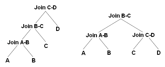
Join ordering and join combination impact a lot when executing a plan. Same with IBM System R, NanoDB only considers left-depth trees.

In NanoDB, we use a dynamic-programming approach to optimize join. The details are as following:

1. From FROM-clause and WHERE-clause, planner extracts conjuncts, and constructs leaf nodes (base table, outer join, subquery). If it is possible to apply predicate to a leaf node, then apply it.
2. Use dynamic programming to choose the "best" join plan

The DP scheme is as following:

• DP states: Maintain a hash map{leaf nodes sets, join plan}.
• DP init: Leaf nodes
• DP iteration: In i-th iteration, the hash map contains only i#-leaf nodes set, so that we can walk through leaf node to find out whether it is possible to construct a i+1#-leaf nodes set and its join plan. If there is a join plan for a leaf nodes set, always choose the less cost one. (By the way, apply predicate if possible)

for plan_n in JoinPlans_n: # Iterate over plans that join n leaves
 for leaf in LeafPlans: # Iterate over the leaf plans
 if leaf already appears in plan_n:
 continue # This leaf is already joined in by the current plan
​
 plan_n+1 = a new join-plan that joins together plan_n and leaf
 newCost = cost of new plan
 if JoinPlans_n+1 already contains a plan with all leaves in plan_n+1:
 if newCost is cheaper than cost of current "best plan" in JoinPlans_n+1:
 # plan_n+1 is the new "best plan" that combines this set of leaf-plans!
 replace current plan with new plan in JoinPlans_n+1
 else:
 # plan_n+1 is the first plan that combines this set of leaf-plans
 add plan_n+1 to JoinPlans_n+1

Summary

In summary, NanoDB has a naïve cost based optimizer. In the query plan tree, leaf node inherits statistics of a table, while every higher-level node uses its own strategy to estimate plan cost. Finally, optimizer gets the whole cost from root node. The optimizer uses dynamic programming approach to find the best left-depth tree plan.

Published by Tech Blog - Huang Blog.