RadKey: A Sticker Under Your Desk Reads Your Keyboard Through a Concrete Wall - With Attack Code

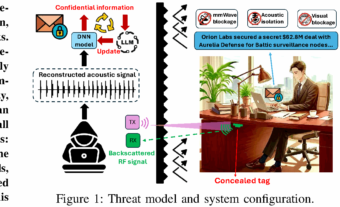
An Inch-Wide Sticker That Hears Every Keystroke

Picture this: there's an inch-wide thing glued under your desk. No battery, no wires, no connection to your keyboard whatsoever. And a reader sits behind the wall, in the next room - reading everything you type. Passwords, messages, search queries. And there's no direct radio path between transmitter and receiver at all - the signal takes a detour, straight through the concrete.

Let me name the thing that surprises me most right up front. The attack is called RadKey, and it was built at Michigan State University (demo video at the link; the work was accepted to IEEE S&P 2026, DOI:10.1109/SP63933.2026.00160) - by two departments working together, Computer Science and Engineering and Radiology. The nastiest part isn't the range and isn't the wall. It's that the attack doesn't need your data. None of it.

Let's take the threat model step by step (the threat model describes who's attacking, what they can do, and what you should expect from them). Inside the room hides a passive RF tag - a small pad on a printed circuit board that gets stuck under the desk. Passive means no power source: it draws energy directly from the radio wave the reader sends out. The reader sits outside, behind the wall, and can be pretty much anywhere within a reasonable radius. To plant the tag, the attacker needs one short moment of physical access - walk into the meeting room, stick it under the tabletop, walk out. From there the sticker lives there for weeks, drawing nothing. The authors show the whole setup in the first figure - tag inside, reader outside, a wall between them.

The victim has to install nothing. The keyboard is never touched, no software, no modifications. It works on a rubber-dome office keyboard, on laptop scissor switches, on a mechanical board - on anything sitting on the same rigid desk as the tag.

And here's the twist that made me sit down and write this in the first place. Classic acoustic keyboard attacks require you to collect a pile of labeled keystrokes from your specific victim on their specific keyboard - otherwise accuracy falls apart. RadKey collects no victim-specific data at all. Zero samples. And accuracy stays high anyway. How does that work? I'll break it down section by section, but the short version: part of the job is done by the clever physics of the radio tag, and part by a language model that fine-tunes the recognizer live, mid-surveillance, feeding it its own guesses as labels.

Code First: How to Reproduce Demodulation and Online Fine-Tuning

The author asked me to show the code implementing the key steps of the attack - and I think that's the right call, because behind the formulas in the paper it's easy to lose sight of the fact that in practice everything boils down to a couple dozen lines of numpy. Let's walk the reader pipeline in exactly the order the signal flows through it.

Some context first. The tag picks up vibration and sound from keystrokes with a piezo sensor (piezo - a material that produces a voltage under mechanical pressure), and it turns that voltage into a frequency shift of its reflected radio signal. So what comes out is classic frequency modulation - FM, exactly like in FM radio, where the voice lives in tiny wobbles of the carrier frequency. Which means to pull the keystroke signal back out, the reader has to measure those frequency wobbles.

FM Demodulation via Phase Difference

The key idea: instantaneous frequency is the time derivative of phase. The phase of a complex signal is its angle on the complex plane, and if we take the phase difference between two adjacent samples (samples - individual measurements of the signal taken at a fixed rate), multiplied by the sampling frequency, we get an estimate of that keystroke signal. This is Equation 12 from the paper.

import numpy as np

def fm_demodulate(baseband, fs, delta):
    # baseband - complex signal after shifting to zero (zero-IF)
    # fs - sampling frequency, delta - carrier modulation coefficient
    phase = np.angle(baseband)                 # instantaneous phase
    dphase = np.diff(np.unwrap(phase))         # phase difference of adjacent samples
    v_s = dphase * fs / (2 * np.pi * delta)    # recovered keystroke signal
    return v_s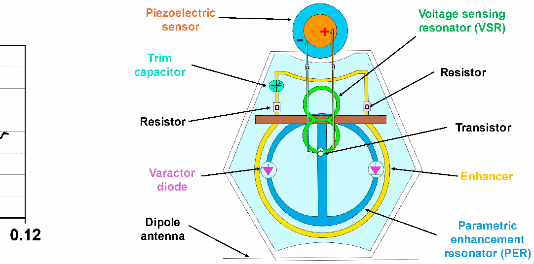

The np.unwrap matters here - phase lives in the range from minus pi to pi and "jumps" across the edge, and unwrap stitches those jumps into a continuous line, otherwise the derivative spits out garbage on every wrap-around.

CFO Correction: Finding Your Own Carrier

The problem is that the reflected signal's frequency doesn't stay put. Because the tag isn't ideal and because of, say, thermal drift, the carrier centers slowly wander - this is called carrier frequency offset (CFO). If you don't correct for it, the demodulation goes off the rails. On top of that, because of manufacturing defects the tag reflects not on one carrier but on several at once, evenly spaced across the spectrum. The authors handle this crudely but effectively - they take the strongest carrier, throw the rest away, and say the quality loss is negligible.

The mechanics are simple: cut the signal into frames, run an FFT (fast Fourier transform - decomposes a signal into its constituent frequencies), find the peak, and shift that peak to zero.

def cfo_correct(x, fs):
    spec = np.fft.fftshift(np.fft.fft(x))
    freqs = np.fft.fftshift(np.fft.fftfreq(len(x), 1/fs))
    f_c0 = freqs[np.argmax(np.abs(spec))]      # strongest carrier frequency
    t = np.arange(len(x)) / fs
    return x * np.exp(-1j * 2 * np.pi * f_c0 * t)  # shift to baseband

There's one detail worth keeping in mind about frequencies. The reflected radio signal first gets shifted down to an intermediate frequency (IF) around 40 kHz - done to escape DC interference and preserve the low-frequency content of the keystrokes. Only afterwards, at the feature extraction stage, the stream gets resampled to 44.1 kHz - the familiar audio rate. The keystroke signal itself is very narrowband, under 40 kHz, and it's precisely this narrowbandness that lets you ignore multipath entirely (multipath - when a signal arrives via several reflected paths and interferes with itself). For FM with such a narrow band the effect is negligible, which makes life noticeably easier.

Segmentation: Where Each Keystroke Begins

Now we have a continuous stream, and we need to slice it into individual keystrokes. The authors compute a short-time energy envelope - how "loud" the signal is within a sliding window (Equation 13). An energy burst = a keystroke.

def energy_envelope(s, L):
    # sliding RMS window of length L
    return np.sqrt(np.convolve(s**2, np.ones(L)/L, mode='same'))

def detect_onsets(s, L, win, lam, min_gap):
    A = energy_envelope(s, L)
    onsets = []
    for n in range(len(A)):
        lo, hi = max(0, n-win), min(len(A), n+win)
        mu = A[lo:hi].mean()          # local mean
        rho = A[lo:hi].std()          # local spread
        if A[n] > mu + lam * rho:     # adaptive threshold mu + lambda*rho
            if not onsets or n - onsets[-1] > min_gap:
                onsets.append(n)
    return onsets

The trick here is the adaptive threshold mu + lambda*rho instead of a fixed one - it adjusts to the local noise level, so segmentation survives varying keystroke loudness and varying tag placement. And min_gap cleans out false triggers from reverberation and hand jitter - within a window we keep only the strongest peak.

LLM as a Source of Pseudo-Labels

Now for the interesting part. Usually a language model gets bolted onto attacks like this after the fact - the classifier spits out garbled text, the LLM tidies it up, done. Here the idea goes deeper: the LLM works as a source of pseudo ground-truth ("supposedly correct" labels the model invents itself, because the attacker has no real ones), and the recognizer fine-tunes on those labels right at runtime. In the prototype this is LLaMA-3.2-3B, run locally - no keystrokes ever leave the machine.

The loss here (loss - the loss function you minimize during training) is hybrid, Equation 15: cross-entropy against the LLM's labels, plus an overconfidence penalty, plus parameter smoothing.

def total_loss(logits, llm_labels, theta, theta_prev,
               l1=1.0, l2=0.3, l3=0.1):
    # NOTE: weights l1/l2/l3 are illustrative; the paper calls them
    # "empirical weights" with no concrete numbers. Signs are shown for clarity.
    # L_LLM-Align: pull toward the labels the LLM gave
    L_align = cross_entropy(logits, llm_labels)
    # L_Conf: entropy regularization. Penalizing overconfidence =
    # REWARDING high entropy, so we ADD the entropy (+l2)
    probs = softmax(logits)
    entropy = -(probs * log(probs)).sum(-1).mean()
    # L_Smooth: don't let weights drift away - guards against catastrophic forgetting
    L_smooth = ((theta - theta_prev) ** 2).sum()
    return l1*L_align + l2*entropy + l3*L_smooth

# online adaptation loop
for window in keystroke_stream:
    feats = extract_features(window)
    logits = classifier(feats)
    text = decode(logits)
    if llm_is_coherent(text):              # coherence check!
        labels = llm_pseudo_label(text)
        loss = total_loss(logits, labels, classifier.theta, theta_prev)
        loss.backward(); optimizer.step()

A small but important caveat about the signs and weights. I set l1=1.0, l2=0.3, l3=0.1 for illustration - in the paper itself they appear as "empirical weights" without concrete numbers, so don't take them as a fact from the work. And a note on entropy: penalizing overconfidence via entropy regularization works by rewarding a high-entropy distribution, so it makes more sense to add the entropy than to subtract it. The point is to keep the model from screaming "I'm 100% sure" out of nowhere and from locking in confident mistakes.

The three terms cover three problems. Cross-entropy pulls the recognizer toward what the language model considers meaningful text. Entropy regularization stops it from locking in confident errors. And smoothing keeps the weights from drifting off and forgetting everything they learned offline - that's the guard against catastrophic forgetting.

But the crucial line is llm_is_coherent(text). Adaptation fires only if the input is meaningful. The prompt asks the LLM to judge whether the decoded text looks like normal human speech, and only if it does - only then do we fine-tune on it. Why? To avoid poisoning the model on a password. If someone hammers out x7$kQ2!p, there's no linguistic meaning there at all, and feeding that in as a label means breaking the classifier. The coherence check screens out such inputs and stops the attack from shooting itself in the foot.

Two Resonators and a Chunk of Piezo: How the Gadget Modulates Sound into Radio

Now for the hardware - because the whole trick is that a passive inch-wide pad can turn desk vibration into a radio signal, and one that punches through a wall at that.

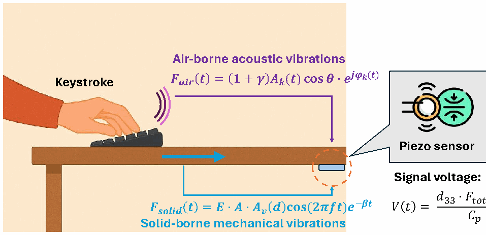
Start with the piezo sensor. When you press a key, it isn't one event but several mechanical ones: the finger touches the keycap, the key bottoms out, and it springs back. On the oscillogram of a single keystroke you see three peaks - the touch peak, the hit peak (bottoming out), and the release peak. Each of these events produces both airborne sound and vibration traveling through the desk. The piezo catches the superposition of both and outputs a voltage. An important fact we'll come back to: the signal reaches the tag via two different paths - through the solid body and through the air. For now just remember there are two paths.

That voltage then goes into the VSR - the voltage sensing resonator. It's an LC circuit (a coil plus a capacitor, which has its own resonant frequency), where the role of the capacitor is played by a varactor - a diode whose capacitance depends on the applied voltage. The piezo voltage changes the varactor's capacitance, the capacitance changes the circuit's resonant frequency. And here's the key point the authors formalize in Theorem 1: at small voltages the relationship between voltage and frequency shift is almost linear. So the tag performs frequency modulation of the sound entirely in the analog domain, with no digitization at all - which simplifies demodulation on the reader side later on.

The second resonator is the PER - the parametric enhancement resonator. It's magnetically coupled to the VSR and solves two problems. First, it pumps energy out of the reader's signal to sustain resonance (again, there's no battery). Second, and more importantly, it separates the excitation and reflection frequencies.

Here's why that matters. Ordinary RFID has a headache called self-interference: the tag reflects on the same frequency it's illuminated on, and the powerful excitation signal drowns out the weak reflected one - the reader simply can't hear the response. The PER solves this through two resonance modes at once: circular and butterfly. The butterfly mode takes the excitation from the reader, the circular mode is magnetically coupled to the VSR and re-radiates the backscatter at the reflection frequency, and their frequencies differ. On the spectrogram of the received signal you see a clean separation: excitation in one place, the reflected keystroke signal in another. Self-interference goes away, and range grows with it.

The prototype specifics: the tag is excited at 915 MHz, and it reflects at 515 MHz. The low frequency is chosen deliberately - it passes through walls far better and generally behaves more nicely during propagation. The excitation is driven by a USRP N310 (a software-defined radio) through a power amplifier, at 30 dBm. The PER is etched on a 0.8 mm G10 substrate (glass-epoxy laminate) with an inner diameter of 13.5 mm, and the whole assembly fits on an inch-wide board. The authors show the tag schematic with all four elements - piezo, VSR, PER, and dipole antenna - in a separate figure.

And the final touch that hooked me most. The authors ran an isolation experiment: they put the keyboard and the tag on separate desks so vibration physically couldn't reach the tag through a solid body. And the tag still caught the keystrokes - through the airborne acoustic channel, via that air-borne path. The piezo turned out to be sensitive enough to sound in the air, not just to desk vibration. Which means even without a mechanical link, the tag keeps hearing the keyboard.

TDoA: Why the Attack Works on a Stranger's Keyboard and a Stranger's Fingers

Now we reach the part that grabs me most in this work - how the attack manages without a single sample of the victim's data. The answer hides in the physics of the two paths I mentioned in the hardware section.

When you press a key, the signal reaches the tag along two routes at different speeds. Vibration travels through the desk - the solid-borne path, fast, because sound travels quickly in a solid body. Acoustics travel through the air - the air-borne path, slow, around 340 m/s. So the same keystroke arrives at the piezo twice, with a small delay between arrivals.

That delay is called TDoA - Time Difference of Arrival. And here's the beauty of it: TDoA is determined mostly by geometry - the distance between the key, the desk, and the tag, plus the speed of sound in wood and in air. Not by how hard you hit the keys, how fast you type, or how you hold your hands. So the feature is almost invariant to the user and the keyboard. That's exactly what carries the generalization - a model trained on some people works on others.

But there's a subtlety in how you feed this TDoA to a neural network. You could compute a single number - the delay in milliseconds - via cross-correlation. The problem is that one scalar number is wildly sensitive to noise and interference. So the authors do something cleverer: they turn the TDoA into a picture. They take a window around the hit peak and run it through time-frequency transforms - a Mel spectrogram (a representation of sound by time and frequency, tuned to human hearing) and a CWT (wavelet transform, good at catching short, sharp events). The delay between the two paths gets baked into subtle desynchronizations and structural differences in these pictures. Such a distributed representation is far more robust to noise than a single number.

From there they work at two scales. Coarse-grained features take the whole keystroke, a window of about 330 milliseconds, to capture the entire acoustic autograph: touch, hit, release, reverberation. These are extracted by a CoAtNet backbone (a hybrid of convolutions and attention - convolutions catch local patterns, attention models long-range dependencies). Fine-grained features live in a narrow window around the hit peak and hold those TDoA pictures. The two streams merge through cross-attention (a mechanism that decides for itself which features matter more right now - the global shape or the fine peak details).

They tested this honestly, cross-user: the model was trained on one group of people and tested on completely different, previously unseen ones. Ten people with different typing styles and speeds took part in the experiments overall. And here's the payoff the whole thing was built for: 4-8 samples per key from strangers is enough - not from the victim. And without the LLM, training hits a plateau after roughly 20 samples per key - more data doesn't help. With the language model, the system reaches high accuracy already at 4-8 samples. Physics provides the invariant feature, the LLM finishes off the rest.

Numbers Worth Sending Your Colleagues: 8 Meters, Concrete, and +10% From the LLM

Now the numbers - the ones you want to drop into the team chat with the caption "just look at this."

Start with tag-reader range (Table 3 in the paper). At one meter, RadKey delivers an F1-score of 98.3% and a character error rate (CER - the fraction of wrong characters, lower is better) of just 1.2%. Makes sense, it's close. More interesting is what happens at eight meters, especially once furniture blocks the line of sight past six meters: F1 holds at 90.5%, CER at 5.1%. Eight meters, obstacles, and key recognition accuracy still above ninety percent.

Now switch off the LLM and watch what happens. Past 5 meters everything starts falling apart: at 6 meters CER jumps to 14.6%, at 8 meters to 23.7%. Nearly every fourth character wrong. So the tag physics alone stretches to about five meters, and beyond that the weak signal is carried entirely by the language model. The difference between 5.1% and 23.7% at the same distance is precisely the LLM's contribution.

There's a second range axis too - the distance between the tag and the keyboard (Table 2), varied from 10 to 120 cm. Here the degradation is gradual: the farther the tag from the keys, the weaker the vibration and the lower the SNR. Without the LLM, at 120 cm CER creeps up to 9.3%, while with online adaptation it stays around 2.7% - meaning you can hide the tag more than a meter from the keyboard and the attack still works. Handy for stealth: you don't have to glue the pad directly under the keys.

Through the wall is its own show. Fifteen centimeters of concrete, reader outside, fully non-line-of-sight, the direct radio path blocked solid. And key recognition accuracy holds high. Three things converge here: the noise- and fading-resistance of the dual-resonator frequency modulation, the two-path sensing that doesn't collapse when one of the paths is blocked, and the same LLM online adaptation correcting the distortions from passing through concrete.

On the language model's contribution by input type (Table 1). On meaningful text, LLM adaptation lifts accuracy from 84.8% to 97.7% - nearly thirteen points, because natural language gives a pile of semantic hints about where to correct. On passwords and random strings the gain is more modest, from 80.1% to 88.3% - and that's expected, there are barely any linguistic priors there. But even so, the attack squeezes out eight extra points because a classifier fine-tuned on meaningful text then works more accurately on nonsense too.

The ablation chain (turning components on one at a time to see how much each contributes, Table 4) shows each piece's contribution plainly. Coarse features only - F1 63.9%. Add the fine TDoA features - 82.4%, a jump of nearly twenty points, and there's the price of the dual path. LLM after the fact to fix the text - 86.7%. And online adaptation in the training loop - 97.8%, with CER dropping to 1.5%. The difference between "LLM tidies up the output" and "LLM fine-tunes the recognizer" is more than ten F1 points.

And some context for the headline number. The final RadKey configuration gives a Precision of 98.1% (in the paper this is specifically the precision of the final build from the ablation and comparison Table 5, not some abstract "overall accuracy"). Now, what to place it next to. In Table 5 the authors compile about eighteen prior works, and here are a couple of representative ones: acoustics from Zhu et al. - 72.2% from a phone microphone at 25 cm; Liu et al. - 97.7%, but a microphone at 5 cm and a vocabulary limited to a-z; the classic Asonov and Agrawal - 79% from a single microphone at a meter; WiKey on WiFi CSI - 96.4%, but requiring a multi-antenna setup at 30 cm; Chen et al. on 2.4 GHz - 91.8% at five meters with an SDR-FPGA-five-antenna rig. Practically all of them required victim data, often worked on a closed vocabulary, and needed a sensor right under your nose. RadKey does the whole keyboard, eight meters, through concrete, all without victim data.

Five keyboard types, surfaces of glass, wood, and plastic - confidently above ninety everywhere. A nice detail about surfaces: without adaptation it works best on glass - rigid and homogeneous, vibrations reach it with almost no loss; worst on plastic, which dampens things. But with the LLM the difference between surfaces almost vanishes.

What to Do About It and Why It Changes the Rules of the Game

Step back a bit, and RadKey is interesting because it stitches two things into one pipeline that usually live in separate worlds: passive RF physics and supervision from a language model. The division of labor between them was already covered earlier.

To my mind, the main shift is exactly the thing discussed earlier. Before, there was a natural barrier - want to read someone's keyboard, then go train your model on their keystrokes first. The combination of a physical invariant and language priors removes that barrier. The attack has become scalable in a way it wasn't before.

Defense, laid out by layers, breaks in four places. At the physical level, damping works: acoustic foam, rubber mats, vibration-absorbing pads under the desk kill the vibration and sound before they ever reach the tag. At the signal level, a defender can actively interfere - inject controlled vibrations during typing, generate background RF noise, and set fingerprinting traps that monitor backscatter and flag suspicious passive tags by their anomalous reflection and resonance characteristics. At the semantic level, the LLM's language priors break down - if the input doesn't look like natural text, the model has nothing to grab onto. Hence input randomization, decoy keystrokes, and on-screen keyboards with randomized key layouts: they tear apart the very coherence the prompt checks before launching adaptation. Password managers, by the way, pull in the same direction - a random string hands the language model not a single hint.

And the fourth layer is proactive, built into the system architecture: trusted computing modules that catch unauthorized sensor hardware, sensor access control policies that flag anomalous passive tags, and adversarial-learning models that deliberately break LLM inference in a hostile environment. The tag itself, incidentally, isn't invisible - it can be found by visual inspection, and the reader's RF activity is caught by spectral monitoring.

So the vector I'd keep in mind: a new sensor plus LLM post-processing. Their pairing specifically, rather than the radio tag or the language model on its own. It seems like there'll only be more hybrids like this going forward.

Research reference: https://arxiv.org/abs/2606.10148