Point Spread Function

🛑 ALL INFORMATION CLICK HERE 👈🏻👈🏻👈🏻
Point Spread Function
Home
Solutions
Basic Microscopy
The Point Spread Function
Resources
Basic Microscopy
About Us
Download Portal
Subscribe to Newsletter
About ZEISS
Career
Press & Media
Publisher
Legal Notice
Data Protection
Cookie Preferences
The ideal point spread function (PSF) is the three-dimensional diffraction pattern of light emitted from an infinitely small point source in the specimen and transmitted to the image plane through a high numerical aperture (NA) objective. It is considered to be the fundamental unit of an image in theoretical models of image formation. When light is emitted from such a point object, a fraction of it is collected by the objective and focused at a corresponding point in the image plane. However, the objective lens does not focus the emitted light to an infinitely small point in the image plane. Rather, light waves converge and interfere at the focal point to produce a diffraction pattern of concentric rings of light surrounding a central, bright disk, when viewed in the x-y plane. The radius of disk is determined by the NA, thus the resolving power of an objective lens can be evaluated by measuring the size of the Airy disk (named after George Biddell Airy). The image of the diffraction pattern can be represented as an intensity distribution as shown in Figure 1. The bright central portion of the Airy disk and concentric rings of light correspond to intensity peaks in the distribution. In Figure 1, relative intensity is plotted as a function of spatial position for PSFs from objectives having numerical apertures of 0.3 and 1.3. The full-width at half maximum (FWHM) is indicated for the lower NA objective along with the Rayleigh limit.
In a perfect lens with no spherical aberration the diffraction pattern at the paraxial (perfect) focal point is both symmetrical and periodic in the lateral and axial planes. When viewed in either axial meridian (x-y or y-z) the diffraction image can have various shapes depending on the type of instrument used (i.e. widefield, confocal, or multiphoton) but is often hourglass or football-shaped. The point spread function is generated from the z series of optical sections and can be used to evaluate the axial resolution. As with lateral resolution, the minimum distance the diffraction images of two points can approach each other and still be resolved is the axial resolution limit. The image data are represented as an axial intensity distribution in which the minimum resolvable distance is defined as the first minimum of the distribution curve.
The PSF is often measured using a fluorescent bead embedded in a gel that approximates an infinitely small point object in a homogeneous medium. However, thick biological specimens are far from homogeneous. Differing refractive indices of cell materials, tissues, or structures in and around the focal plane can diffract light and result in a PSF that deviates from design specification, fluorescent bead determination or the calculated, theoretical PSF. A number of approaches to this problem have been suggested including comparison of theoretical and empirical PSFs, embedding a fluorescent microsphere in the specimen or measuring the PSF using a subresolution object native to the specimen.
The PSF is valuable not only for determining the resolution performance of different objectives and imaging systems, but also as a fundamental concept used in deconvolution. Deconvolution is a mathematical transformation of image data that reduces out of focus light or blur. Blurring is a significant source of image degradation in three-dimensional (3D) widefield fluorescence microscopy. It is nonrandom and arises within the optical train and specimen, largely as a result of diffraction. A computational model of the blurring process, based on the convolution of a point object and its PSF, can be used to deconvolve or reassign out of focus light back to its point of origin. Deconvolution is used most often in 3D widefield imaging. However, even images produced with confocal, spinning disk, and multiphoton microscopes can be improved using image restoration algorithms.
Image formation begins with the assumptions that the process is linear and shift invariant. If the sum of the images of two discrete objects is identical to the image of the combined object, the condition of linearity is met, providing the detector is linear, and quenching and self-absorption by fluorophores is minimized. When the process is shift invariant, the image of a point object will be the same everywhere in the field of view. Shift invariance is an ideal condition that no real imaging system meets. Nevertheless, the assumption is reasonable for high quality research instruments.
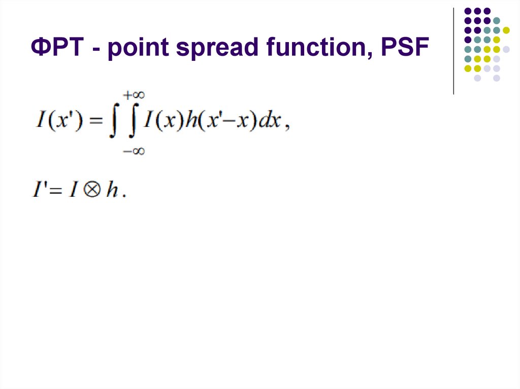
Convolution mathematically describes the relationship between the specimen and its optical image. Each point object in the specimen is represented by a blurred image of the object (the PSF) in the image plane. An image consists of the sum of each PSF multiplied by a function representing the intensity of light emanating from its corresponding point object:
i(x) = o(x - x') × psf(x')dx'(1)
A pixel blurring kernel is used in convolution operations to enhance the contrast of edges and boundaries and the higher spatial frequencies in an image. Figure 2 illustrates the convolution operation using a 3 x 3 kernel to convolve a 6 x 6 pixel object. Above the arrays in Figure 2 are profiles demonstrating the maximum projection of the two-dimensional grids when viewed from above.
An image is a convolution of the object and the PSF and can be symbolically represented as follows:
image(r) = object(r) ⊗ psf(r)(2)
where the image, object, and PSF are denoted as functions of position (r) or an x, y, z and t (time) coordinate. The Fourier transform shows the frequency and amplitude relationship between the object and point spread function, converting the space variant function to a frequency variant function. Because convolution in the spatial domain is equal to multiplication in the frequency domain, convolutions are more easily manipulated by taking their Fourier transform (F).
F{i(x,y,z,t)} = F{o(x,y,z,t)} × F{psf(x,y,z,t)}(3)
In the spatial domain described by the PSF, a specimen is a collection of point objects and the image is a superposition or sum of point source images. The frequency domain is characterized by the optical transfer function (OTF). The OTF is the Fourier transform of the PSF and describes how spatial frequency is affected by blurring. In the frequency domain, the specimen is equivalent to the superposition of sine and cosine functions, and the image consists of the sum of weighted sine and cosine functions. The Fourier transform further simplifies the representation of the convolved object and image such that the transform of the image is equal to the specimen multiplied by the OTF. The microscope passes low frequency (large, smooth) components best, intermediate frequencies are attenuated, and high frequencies greater than 2NA/λ are excluded. Deconvolution algorithms are therefore required to augment high spatial frequency components.
Theoretically, it should be possible to reverse the convolution of object and PSF by taking the inverse of the Fourier transformed functions. However, deconvolution increases noise, which exists at all frequencies in the image. Beyond half the Nyquist sampling frequency no useful data are retained, but noise is nevertheless amplified by deconvolution. Contemporary image restoration algorithms use additional assumptions about the object such as smoothness or non-negative value and incorporate information about the noise process to avoid some of the noise related limitations.
Deconvolution algorithms are of two basic types. Deblurring algorithms use the PSF to estimate blur then subtract it by applying the computational operation to each optical section in a z-series. Algorithms of this type include nearest neighbor, multi neighbor, no neighbor, and unsharp masking. The more commonly used nearest neighbor algorithm estimates and subtracts blur from z sections above and below the section to be sharpened. While these run quickly and use less computer memory, they don't account for cross-talk between distant optical sections. Deblurring algorithms may decrease the signal-to-noise ratio (SNR) by adding noise from multiple planes. Images of objects whose PSFs overlap in the paraxial plane can often be sharpened by deconvolution, however, at the cost of displacement of the PSF. Deblurring algorithms introduce artifacts or changes in the relative intensities of pixels and thus cannot be used for morphometric measurements, quantitative intensity determinations or intensity ratio calculations.
Image restoration algorithms use a variety of methods to reassign out-of-focus light to its proper position in the image. These include inverse filter types such as Wiener deconvolution or linear least squares, constrained iterative methods such as Jansson van Cittert, statistical image restoration, and blind deconvolution. Constrained deconvolution imposes limitations by excluding non-negative pixels and placing finite limits on size or fluorescent emission, for example. An estimation of the specimen is made and an image calculated and compared to the recorded image. If the estimation is correct, constraints are enforced and unwanted features are excluded. This process is convenient to iterative methods that repeat the constraint algorithm many times. The Jansson van Cittert algorithm predicts an image, applies constraints, and calculates a weighted error that is used to produce a new image estimate for multiple iterations. This algorithm has been effective in reducing high frequency noise.
Blind deconvolution does not use a calculated or measured PSF but rather, calculates the most probable combination of object and PSF for a given data set. This method is also iterative and has been successfully applied to confocal images. Actual PSFs are degraded by the varying refractive indices of heterogeneous specimens. In laser scanning confocal microscopy, where light levels are typically low, this effect is compounded. Blind deconvolution reconstructs both the PSF and the deconvolved image data. Compared with deblurring algorithms, image restoration methods are faster, frequently result in better image quality, and are amenable to quantitative analysis.
Deconvolution performs its operations using floating point numbers and consequently, uses large amounts of computing power. Four bytes per pixel are required, which translates to 64 Mb for a 512 x 512 x 64 image stack. Deconvolution is also CPU intensive, and large data sets with numerous iterations may take several hours to produce a fully restored image depending on processor speed. Choosing an appropriate deconvolution algorithm involves determining a delicate balance of resolution, processing speed, and noise that is correct for a particular application.
Rudi Rottenfusser - Zeiss Microscopy Consultant, 46 Landfall, Falmouth, Massachusetts, 02540.
Erin E. Wilson and Michael W. Davidson - National High Magnetic Field Laboratory, 1800 East Paul Dirac Dr., The Florida State University, Tallahassee, Florida, 32310.
Not all products are available in every country. Use of products for medical diagnostic, therapeutic or treatment purposes may be limited by local regulations. Contact your local ZEISS provider for more information.
Point spread function | Словари и энциклопедии на Академике
The Point Spread Function in Details
Point Spread Function - an overview | ScienceDirect Topics
A Beginners Guide to The Point Spread Function
Point spread function ( psf )
(1.1) R = ( x ′ − x ) 2 + ( y ′ − y ) 2 + z 0 2 .
(1.2) R 0 = x ′ 2 + y ′ 2 + z 0 2 .
(1.3) h ( x , y ) = b ∫ ∫ P ( x ′ , y ′ ) e − j ( ϕ − ϕ 0 ) R d x ′ d y ′ ,
(1.4) h ( x , y ) = D e − j k ( x 2 + y 2 ) / 2 z 0 ∫ ∫ P ( x ′ , y ′ ) e j k n ( x x ′ + y y ′ ) / z 0 d x ′ d y ′ .
(1.5) h ( x , y ) = D ∫ ∫ P ( x ′ , y ′ ) e j k n ( x x ′ + y y ′ ) / z 0 d x ′ d y ′ .
(1.7) d r ( 3 dB ) = 0.51 λ n sin θ 0 = 0.51 λ N . A . .
(7.52) v ( x , y ) = u ( x , y ) a ( x , y ) e j ϕ ( x , y )
(7.53) w ( x , y ) = h ( x , y ) * v ( x , y ) .
(7.54) v ( x , y ) = undefined v R ( x , y ) + j v I ( x , y )
(7.55) w ( x , y ) = w R ( x , y ) + j w I ( x , y ) .
(7.56) w R ( x , y ) = ∫ − ∞ ∞ ∫ − ∞ ∞ h ( α , β ) v R ( x − α , y − β ) d α d β
(7.57) f ( x , y ) = w R ( x , y ) 2 + w I ( x , y ) 2 .
(7.58) Pr [ f ( x , y ) ≤ f ] = ∫ 0 2 π ∫ 0 f 0.5 1 2 π σ 2 e − ρ / 2 σ 2 ρ d ρ d ϕ
(7.60) p f ( f ) = { 1 g e − f / g f ≥ 0 0 f < 0 ,
(7.61) f ( x , y ) = g ( x , y ) q ,
(7.62) p q ( x ) = { e − x x ≥ 0 0 x < 0.
(7.63) f ^ ( x , y ) = 1 M ∑ i = 1 M undefined f i ( x , y )
(7.64) = g ( x , y ) ∑ i = 1 M q i ( x , y ) M .
(10.2.19) I 0 = f π D 2 ( 1 − ɛ 2 ) 4 λ 2 f 2 = π f ( 1 − ɛ 2 ) 4 λ 2 F 2 ⋅
(10.2.20) 〈 I ( disk ) 〉 = σ f π r 1 2 = σ f π γ 2 ( 1 ⋅ 22 λ F ) 2 ,
(10.2.21) 〈 I ( disk ) 〉 I 0 = 4 σ ( 1 ⋅ 22 π γ ) 2 ( 1 − ɛ 2 ) = 0 ⋅ 272 σ γ 2 ( 1 − ɛ 2 ) ⋅
s = p ⊗ ⊗ f + n = ∫ − X X ∫ − Y Y p ( x − x ′ , y − y ′ ) f ( x ′ , y ′ ) d x ′ d y ′ + n ( x + y ) .
s i j = p i j ⊗ ⊗ f i j + n i j = ∑ n ∑ m p i − n , j − m f n m + n i j
∑ n ≡ ∑ n = − N N and ∑ m ≡ ∑ m = − M M .
Point spread functions tend to have higher values at their origins, since the influence of the point where they are applied is nearly always predominant;
The Point Spread Function and Pupil Function The performance of an imaging system can be quantified by calculating its point spread function (PSF). The amplitude PSF, h ( x,y ), of a lens is defined as the transverse spatial variation of the amplitude of the image received at the detector plane when the lens is illuminated by a perfect point source. Diffraction coupled with aberrations in the lens will cause the image of a perfect point to be smeared out into a blur spot occupying a finite area of the image plane. For a simple lens the concept of reciprocity applies, so that the function h ( x,y ) also denotes the amplitude variation at the focal plane when the lens is illuminated using a point source. In the same way, the intensity PSF, I h ( x,y ) = | h ( x,y )| 2 , of an objective is defined as the spatial variation of the intensity of the image received at the detector plane when the lens is illuminated by a perfect point source.
The definition of the PSF has it origin in linear systems theory. Its properties include the principle that for a linear spatially invariant imaging system, the image can be calculated by convolving a function characterizing the transmission t ( x,y ) or reflectivity r ( x,y ) of the sample with the PSF of the system. The analogy in electrical circuit theory is the convolution of an arbitrary signal with the response of a circuit. The PSF is the two-dimensional optical analog of the electrical impulse response of a circuit to a delta function input or infinitesimally narrow pulse.
The PSF is given in the paraxial approximation by the Fourier transform of the pupil function of the lens. To illustrate this mathematical relationship, we consider a beam of unit amplitude passing through the objective lens which is focused to a point P 0 at (0,0, z 0 ) on the axis, of the lens as illustrated in Fig. 1.8 . The pupil function of the objective, P ( x′ , y ′), is defined as the amplitude attenuation of the beam passing through the lens at a point ( x′,y′,0 ), on the plane D 2 just in front of the lens. The distance from the point S to the point P at ( x,y,z 0 ) on the focal plane is
Figure 1.8 . Schematic of the variables used in calculation of PSF in a standard optical microscope.
Similarly, the distance from S to the focal point P 0 is
All the rays reaching the point P 0 will be in phase if the lens introduces a phase delay ϕ 0 = A – knR 0 at each point ( x′,y′ ,0), where k = 2π/λ. In these expressions, λ is the free-space wavelength, n the refractive index of the medium between the lens and the point P 0 , and A a constant. In this case the phase change along the ray of length R is ϕ = knR.
Rayleigh-Sommerfeld diffraction theory can be used to calculate the scalar potential of the beam at the point ( x,y,z 0 ). For a simple lens the scalar potential is just the amplitude PSF of the lens, 8 , 9
To express Eq. (1.3) as a Fourier transform relation, the phase term is expanded to second order in x / z 0 , y / z 0 , x′ / z 0 , and y′ / Z 0 using the paraxial approximation, z 0 ≫ x′, z 0 ≫ y′, z 0 ≫ x , and z 0 ≫ y. Setting R ≈ z 0 in the denominator of the integrand, the equation becomes
In Eq. (1.4) D is a constant that is normally chosen to make the maximum value of h ( x,y ) equal to unity.
Finally, assuming that the spot size is small, the exponential term in front of the integral is unity so that
It is clear from Eq. (1.5) that the amplitude PSF of a simple lens at the focus is proportional to the Fourier transform of the pupil function.
Point Spread Function of a Spherical Lens In this book we will use the notation h ( r ) for the radial variation of the amplitude PSF of a circularly symmetric aberration-free lens, where r is the distance from the center point of the image. If the pupil function is uniform, it can be shown from Eq. (1.5) in the paraxial approximation that h ( r ) has the form of the Airy function 8 , 10
In Eq. (1.6) , the normalized distance from the optical axis of the system is defined as ν = krn sin θ 0 = kr ( N.A. ), where k = 2π/λ is the wave number, λ is the free-space wavelength, and J 1 (ν) is a Bessel function of the first order and the first kind. The amplitude and intensity of the Airy function are plotted in Fig. 1.9 . It will be noted that the amplitude is maximum at ν = 0 and that there are subsidiary minima and maxima or sidelobes. The first zero of the response is located at ν = 3.832 or r = 0.61λ/ n sin θ 0 . The first sidelobe or maximum in the amplitude response is at ν = 5.136 or r = 0.82λ/n sin θ 0 and is reduced in amplitude by 0.132 or −;17.6 dBs from the amplitude at the center of the main lobe. The amplitude PSF is related directly to the electric field at the sample, whereas the intensity PSF is related to the power per unit area or the square of the electric field.
Figure 1.9 . The amplitude variation (dotted line) and intensity (solid line) for the PSF of a simple lens.
The width between the half-power points of the main lobe, d r ( 3 dB), in the intensity response is known as the full width at half-maximum (FWHM) or 3-dB width and is given by the formula
This formula for the width of the image of a point object is also called the single point resolution of the standard optical microscope.
The resolution of an optical microscope can be improved by using liquid immersion objectives. These lenses use a high-refractive-index liquid between the sample and the microscope objective. Surrounding the sample with a high-index material reduces the effective wavelength in the medium, thereby improving the resolution. Two commonly used immersion fluids are water ( n = 1.33) and immersion oil ( n = 1.52). Water is often used for biological imaging when no cover glass is present on the sample. Oil is used for most other samples because its index most closely matches that of the cover glass, thus minimizing reflections from this surface and avoiding aberrations induced by the glass. Throughout this text, as is the common practice, objective lenses will be specified by both their magnification and their numerical aperture, for example, 80×/0.95 N.A.
Jonathan M. Blackledge , in Digital Image Processing , 2005
The point spread function associated with the back-projection function is | r | −1 which has a Fourier transform of the same form, i.e. | k | −1 . The inverse filter is therefore given by | k |. Fortunately, this particular filter is non-singular and can therefore be used directly to deconvolve the back-projection function without recourse to optimization methods such as the Wiener filter. This is a rare and exceptional case. The process for deconvolving the back-projection function is relatively straightforward. The 2D Fourier transform of this function is taken and the real and imaginary parts multiplied by | k |. The inverse Fourier transform is then computed, the reconstruction being given by the real part of the output.
Speckle is one of the more complex image noise models. It is signal dependent, non-Gaussian, and spatially dependent. Much of this discussion is taken from [ 14 , 15 ]. We will first discuss the origins of speckle, then derive the first-order density of speckle, and conclude this section with a discussion of the second-order properties of speckle.
In coherent light imaging, an object is illuminated by a coherent source, usually a laser or a radar transmitter. For the remainder of this discussion, we will consider the illuminant to be a light source, e.g., a laser, but the principles apply to radar imaging as well.
When coherent light strikes a surface, it is reflected back. Due to the microscopic variations in the surface roughness within one pixel, the received signal is subjected to random variations in phase and amplitude. Some of these variations in phase add constructively, resulting in strong intensities, and others add deconstructively, resulting in low intensities. This variation is called speckle .
Of crucial importance in the understanding of speckle is the point spread function of the optical system. There are three regimes:
The point spread function is so narrow that the individual variations in surface roughness can be resolved. The reflections off the surface are random (if, indeed, we can model the surface roughness as random in this regime), but we cannot appeal to the central limit theorem to argue that the reflected signal amplitudes are Gaussian. Since this case is uncommon in most applications, we will ignore it.
The point spread function is broad compared to the feature size of the surface roughness, but small compared to the features of interest in the image. This is a common case and leads to the conclusion, presented below, that the noise is exponentially distributed and uncorrelated on the scale of the features in the image. Also, in this situation, the noise is often modeled as multiplicative.
The point spread function is broad compared to both the feature size of the object and the feature size of the surface roughness. Here, the speckle is correlated and its size distribution is interesting and is determined by the point spread function.
The development will proceed in two parts. Firstly, we will derive the first-order probability density of speckle and, secondly, we will discuss the correlation properties of speckle.
In any given macroscopic area, there are many microscopic variations in the surface roughness. Rather than trying to characterize the surface, we will content ourselves with finding a statistical description of the speckle.
We will make the (standard) assumptions that the surface is very rough on the scale of the optical wavelengths. This roughness means that each microscopic reflector in the surface is at a random height (distance from the observer) and a random orientation with respect to the incoming polarization field. These random reflectors introduce random changes in the reflected signal's amplitude, phase, and polarization. Further, we assume these variations at any given point are independent from each other and independent from the changes at any other point.
These assumptions amount to assuming that the system cannot resolve the variations in roughness. This is generally true in optical systems, but may not be so in some radar applications.
The above assumptions on the physics of the situation can be translated to statistical equivalents: the amplitude of the reflected signal at any point, ( x , y ), is multiplied by a random amplitude, denoted a ( x , y ), and the polarization, ϕ ( x , y ) , is uniformly distributed between 0 and 2π.
Let u ( x , y ) be the complex phasor of the incident wave at a point ( x , y ), v ( x , y ) be the reflected signal, and w ( x , y ) be the received phasor. From the above assumptions,
and, letting h ( · , · ) denote the 2D point spread function of the optical system,
One can convert the phasors to rectangular coordinates:
Since the change in polarization is uniform between 0 and 2 π , v R ( x , y ) and v I ( x , y ) are statistically independent. Similarly, w R ( x , y ) and w I ( x , y ) are statistically independent.
The integral in ( 7.56 ) is basically a sum over many tiny increments in x and y . By assumption, the increments are independent of one another. Thus, we can appeal to the central limit theorem and conclude that the distributions of w R ( x , y ) and w I ( x , y ) are each Gaussian with mean 0 and variance σ 2 . Note, this conclusion does not depend on the details of the roughness, as long as the surface is rough on the scale of the wavelength of the incident light and the optical system cannot resolve the individual components of the surface.
The measured intensity, f ( x , y ) , is the squared magnitude of the received phasors:
The distribution of f can be found by integrating the joint density of w R and w I over a circle of radius f 0.5 :
The corresponding density is p f ( f ):
where we have taken the liberty to introduce the mean intensity, g = g ( x , y ) = 2 σ 2 ( x , y ) .
A little rearrangement can put this into a multiplicative noise model:
The mean of q is 1 and the variance is 1.
The exponential density is much heavier tailed than the Gaussian density, meaning that much greater excursions from the mean occur. In particular, the standard deviation of f equals E [ f ], i.e., the typical deviation in the reflected intensity is equal to the typical intensity. It is this large variation that causes speckle to be so objectionable to human observers.
It is sometimes possible to obtain multiple images of the same scene with independent realizations of the speckle pattern, i.e., the speckle in any one image is independent of the speckle in the others. For instance, there may be multiple lasers illuminating the same object from different angles or with different optical frequencies. One means of speckle reduction is to average these images:
Now, the average of the negative exponentials has mean 1 (the same as each individual negative exponential) and variance 1/ M . Thus, the average of the speckle images has a mean equal to g(x,y) and variance g 2 ( x , y )/ M .
Figure 7.10 shows an uncorrelated speckle image of San Francisco. Notice how severely degraded this image is. Careful examination will show that the light areas are noisier than the dark areas. This image was created by generating an “image” of exponential variates and multiplying each by the corresponding pixel value. Intensity values beyond 255 were truncated to 255.
FIGURE 7.10 . San Francisco with uncorrelated speckle.
The correlation structure of speckle is largely determined by the width of the point spread function. As above the real and imaginary components (or, equivalently, the X and Y components) of the reflected wave are independent Gaussian. These components ( w R and w I above) are individually filtered by the point spread function of the imaging system. The intensity image is formed by taking the complex magnitude of the resulting filtered components.
Figure 7.11 shows a correlated speckle image of San Francisco. The image was created by filtering w R and w I with a 2D square filter of size 5 × 5 . This size filter is too big for the fine details in the original image, but is convenient to illustrate the correlated speckle. As above, intensity values beyond 255 were truncated to 255. Notice the correlated structure to the “speckles.” The image has a pebbly appearance.
FIGURE 7.11 . San Francisco with correlated speckle.
We will conclude this discussion with a quote from Goodman [ 16 ]:
The general conclusions to be drawn from these arguments are that, in any speckle pattern, large-scale-size fluctuations are the most populous, and no scale sizes are present beyond a certain small-size cutoff. The distribution of scale sizes in between these limits depends on the autocorrelation function of the object geometry, or on the autocorrelation function of the pupil function of the imaging system in the imaging geometry.
The PSF defined in Section 10.2 .a is a dimensionless measure of the intensity or irradiance of the Airy pattern, but it is also necessary to give physical units to the PSF. In this section we give relations for the irradiance and intensity at the center of the Airy pattern and discuss the average irradiance over the Airy disk.
The terms intensity and irradiance are often interchanged in usage. The definition of irradiance is the energy incident on a surface per unit area per unit time , with units watts/m 2 (W/m 2 ). Physicists commonly use the word intensity for the flow of energy per unit area per unit time through a surface. Astronomers, however, generally follow the definition that intensity is the energy per unit time in a certain direction per unit solid angle , with units watts/steradian (W/sr). We follow this latter usage of intensity. The symbol I is often used to represent both intensity and irradiance, and we follow this convention. The interested reader should consult the reference by Mahajan (1998) for a thorough discussion of the radiometry of imaging.
The relation given in Eq. (10.2.15) is derived by Born and Wolf (1980) . Replacing the energy E in Eq. (10.2.15) by the energy per unit time, or flux f , we have the irradiance I 0 at the peak of the PSF as
It is instructive to compute the peak irradiance for a specific case. Consider a perfect Hubble Space Telescope (HST) with D = 2.4 m, F = 24, ɛ = 0.33, and area A = 4.03 m 2 . Taking the canonical value for the photon flux as 1E4 photons/(sec cm 2 nm) for a zero-magnitude star at λ = 550 nm, we get f = 4.03 E8 photons/(sec nm) = 1.46E-10 W/nm, for the photon and energy flux per nm in the image of the HST with unit transmittance. Substituting the given values into Eq. (10.2.19) , we find I 0 = 1.63E18 photons/(sec m 2 nm) = 0.59 W/(m 2 nm) = 5.9E-13 W/(μm 2 nm), for a zero-magnitude star.
Another quantity of interest is the average irradiance over the Airy disk, that part of the image enclosed by the first dark ring. The average irradiance 〈 I (disk)〉 is the flux in the disk divided by its area, and is given by
where σ is the fraction of the total flux in the Airy disk, r 1 is the radius of the Airy disk, and γ is a numerical factor such that 1.22γ = ω 1 from Table 10.1 for an annular aperture. The value of σ also depends on ɛ, as noted in the discussion of encircled energy in the previous section.
Dividing Eq. (10.2.20) by Eq. (10.2.19) , we get
Taking ɛ = 0 and ɛ = 0.33, we use the results in Table 10.1 and find γ = 1 and γ = 0.9, respectively, and from Table 10.2 we get σ = 0.838 and σ = 0.654, respectively. Putting these values into Eq. (10.2.21) gives 〈 I (disk)〉/ I 0 = 0.228 and 0.246 for the apertures with ɛ = 0 and ɛ = 0.33, respectively, hence a smaller Airy disk roughly compensates for the smaller encircled energy fraction.
For another example assume a passband of 100 nm centered at λ = 550 nm, and a star of apparent magnitude 25 imaged by HST. In this case we find a photon flux of 4.03 photons/sec passing through the HST aperture and 2.63 photons/sec on the Airy disk. Assuming a reflectance of 0.9 for the primary and secondary HST mirrors, a more accurate flux value is approximately 2.1 photons/sec for a star of apparent magnitude 25 at the f /24 focus of HST. The detected photon flux, of course, depends on the efficiency of the optics and detector in a reimaging camera.
As a final item we note that Born and Wolf also define I 0 = EA /λ 2 , hence units are those of intensity rather than irradiance. In this case the integral in Eq. (10.2.13) is over the solid angle subtended by the image at the aperture instead of the area of the image.
D. Arbel , N.S. Kopeika , in Encyclopedia of Modern Optics , 2005
To measure the point spread function (PSF), it is important to determine which size object can be considered a point object. This is affected primarily by instrumentation pixel size. The pixel is the smallest element recordable in image space. The brightness value represents average irradiance over that small portion of the image scene. Pixel size is often related to detector size. If only a portion of the detector is illuminated, the output current is equivalent to that obtained for the same total radiant power absorbed by the detector but averaged over the entire detector area. No detail smaller than a pixel can be resolved in the image. In practice, dead space between pixels violates isoplanaticism (spatial stationarity), which is a requirement for linear systems. Nevertheless, dead space is small and such effects are often neglected in image system characterization. However, it is possible to overcome distortions in MTF measurements arising from this lack of isoplanaticism by using a ‘white’ spatial noise random object. This gives rise to a white noise random image. The ratio of the image power spectral density to object power spectral density is equal to the square of the system MTF. In this way the lack of isoplanaticism is overcome by the spatial randomness of the object and image.
Pixel size strongly affects system MTF. If a pixel represents a point image, then pixel size and shape are minimum spread function. A best case OTF for such an imaging system is then a normalized FT of the pixel shape. For example, a square pixel yields a two-dimensional sinc MTF whose width increases as pixel size decreases.
Jonathan M. Blackledge , in Digital Image Processing , 2005
The fundamental imaging equation for x ∈ [− X , X ], y ∈ [− Y , Y ] is given by
Here, p is the point spread function which describes the way in which information on the object; function f is ‘spread out’ as a result of recording the data. It is a characteristic of the imaging instrument which represents the response of the imaging system to a point source in the object plane and is a deterministic function. The object function f describes the object that is being imaged (its surface or internal structure, for example). The noise n is a non-deterministic function which can at best be described in terms of some statistical distribution. It is a stochastic function which is a consequence of all of the external disturbances that occur during the recording process. The operation ⊗⊗, which denotes 2D convolution, describes the blurring process that occurs when an image is taken. This equation assumes that the imaging system can be described by a stationary process in which the point spread function remains the same over the image domain, i.e. it is spatially invariant. The equation also assumes that the scattering process (e.g. light scattering from a surface) that produces the image is dominated by single scattering events.
For a digital image, we consider a discrete 2D array of space or of space and time and consider the discrete imaging equation given by
Here, the digital image is taken to of size 2 N × 2 M .
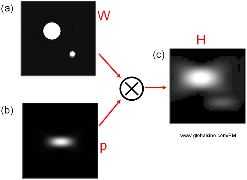
A common application requiring a large PSF is the enhancement of images with unequal illumination. Convolution by separability is an ideal algorithm to carry out this processing. With only a few exceptions, the images seen by the eye are formed from reflected light. This means that a viewed image is equal to the reflectance of the objects multiplied by the ambient illumination. Figure 24-8 shows how this works. Figure (a) represents the reflectance of a scene being viewed, in this case, a series of light and dark bands. Figure (b) illustrates an example illumination signal, the pattern of light falling on (a). As in the real world, the illumination slowly varies over the imaging area. Figure (c) is the image seen by the eye, equal to the reflectance image, (a), multiplied by the illumination image, (b). The regions of poor illumination are difficult to view in (c) for two reasons: they are too dark and their contrast is too low (the difference between the peaks and the valleys).
FIGURE 24-8 . Model of image formation. A viewed image, (c), results from the multiplication of an illumination pattern, (b), by a reflectance pattern, (a). The goal of the image processing is to modify (c) to make it look more like (a). This is performed in Figs. (d), (e) and (f) on the opposite page. Figure (d) is a smoothed version of (c), used as an approximation to the illumination signal. Figure (e) shows an approximation to the reflectance image, created by subtracting the smoothed image from the viewed image. A better approximation is shown in (f), obtained by the nonlinear process of dividing the two images.
To understand how this relates to the problem of everyday vision, imagine you are looking at two identically dressed men. One of them is standing in the bright sunlight, while the other is standing in the shade of a nearby tree. The percent of the incident light reflected from both men is the same. For instance, their faces might reflect 80% of the incident light, their gray shirts 40% and their dark pants 5%. The problem is, the illumination of the two might be, say, ten times different. This makes the image of the man in the shade ten times darker than the person in the sunlight, and the contrast (between the face, shirt, and pants) ten times less.
The goal of the image processing is to flatten the illumination component in the acquired image. In other words, we want the final image to be representative of the objects' reflectance, not the lighting conditions. In terms of Fig. 24-8 , given (c), find (a). This is a nonlinear filtering problem, since the component images were combined by multiplication, not addition. While this separation cannot be performed perfectly, the improvement can be dramatic.
To start, we will convolve image (c) with a large PSF, one-fifth the size of the entire image. The goal is to eliminate the sharp features in (c), resulting in an approximation to the original illumination signal, (b). This is where convolution by separability is used. The exact shape of the PSF is not important, only that it is much wider than the features in the reflectance image. Figure (d) is the result, using a Gaussian filter kernel.
Since a smoothing filter provides an estimate of the illumination image, we will use an edge enhancement filter to find the reflectance image. That is, image (c) will be convolved with a filter kernel consisting of a delta function minus a Gaussian. To reduce execution time, this is done by subtracting the smoothed image in (d) from the original image in (c). Figure (e) shows the result. It doesn't work! While the dark areas have been properly lightened, the contrast in these areas is still terrible.
Linear filtering performs poorly in this application because the reflectance and illumination signals were original combined by multiplication, not addition. Linear filtering cannot correctly separate signals combined by a nonlinear operation. To separate these signals, they must be unmultiplied . In other words, the original image should be divided by the smoothed image, as is shown in (f). This corrects the brightness and restores the contrast to the proper level.
This procedure of dividing the images is closely related to homomorphic processing , previously described in Chapter 22 . Homomorphic processing is a way of handling signals combined through a nonlinear operation. The strategy is to change the nonlinear problem into a linear one, through an appropriate mathematical operation. When two signals are combined by multiplication, homomorphic processing starts by taking the logarithm of the acquired signal. With the identity: log( a × b ) = log( a ) + log( b ), the problem of separating multiplied signals is converted into the problem of separating added signals. For example, after taking the logarithm of the image in (c), a linear high-pass filter can be used to isolate the logarithm of the reflectance image. As before, the quickest way to carry out the high-pass filter is to subtract a smoothed version of the image. The antilogarithm (exponent) is then used to undo the logarithm, resulting in the desired approximation to the reflectance image.
Which is better, dividing or going along the homomorphic path? They are nearly the same, since taking the logarithm and subtracting is equal to dividing. The only difference is the approximation used for the illumination image. One method uses a smoothed version of the acquired image, while the other uses a smoothed version of the logarithm of the acquired image.
This technique of flattening the illumination signal is so useful it has been incorporated into the neural structure of the eye. The processing in the middle layer of the retina was previously described as an edge enhancement or high-pass filter. While this is true, it doesn't tell the whole story. The first layer of the eye is nonlinear, approximately taking the logarithm of the incoming image. This makes the eye a homomorphic processor. Just as described above, the logarithm followed by a linear edge enhancement filter flattens the illumination component, allowing the eye to see under poor lighting conditions. Another interesting use of homomorphic processing occurs in photography. The density (darkness) of a negative is equal to the logarithm of the brightness in the final photograph. This means that any manipulation of the negative during the development stage is a type of homomorphic processing.
Before leaving this example, there is a nuisance that needs to be mentioned. As discussed in Chapter 6 , when an N point signal is convolved with an M point filter kernel, the resulting signal is N + M −1 points long. Likewise, when an M × M image is convolved with an N × N filter kernel, the result is an ( M + N −1) × ( M + N −1) image. The problem is, it is often difficult to manage a changing image size. For instance, the allocated memory must change, the video display must be adjusted, the array indexing may need altering, etc. The common way around this is to ignore it; if we start with a 512 × 512 image, we want to end up with a 512 × 512 image. The pixels that do not fit within the original boundaries are discarded.
While this keeps the image size the same, it doesn't solve the whole problem; these is still the boundary condition for convolution. For example, imagine trying to calculate the pixel at the upper-right corner of (d). This is done by centering the Gaussian PSF on the upper-right corner of (c). Each pixel in (c) is then multiplied by the corresponding pixel in the overlaying PSF, and the products are added. The problem is, three-quarters of the PSF lies outside the defined image. The easiest approach is to assign the undefined pixels a value of zero. This is how (d) was created, accounting for the dark band around the perimeter of the image. That is, the brightness smoothly decreases to the pixel value of zero, exterior to the defined image.
Fortunately, this dark region around the boarder can be corrected (although it hasn't been in this example). This is done by dividing each pixel in (d) by a correction factor. The correction factor is the fraction of the PSF that was immersed in the input image when the pixel was calculated. That is, to correct an individual pixel in (d), imagine that the PSF is centered on the corresponding pixel in (c). For example, the upper-right pixel in (c) results from only 25% of the PSF overlapping the input image. Therefore, correct this pixel in (d) by dividing it by a factor of 0.25. This means that the pixels in the center of (d) will not be changed, but the dark pixels around the perimeter will be brightened. To find the correction factors, imagine convolving the filter kernel with an image having all the pixel values equal to one . The pixels in the resulting image are the correction factors needed to eliminate the edge effect.
T. Ritschel , in High Dynamic Range Video , 2016
The output image is convolved with the colored PSF computed in the previous step. This is different from previous methods, which used only billboards composed onto single bright pixels. Use of the FT convolution theorem allows one to compute the convolution as the multiplication of the FFT of the PSF and an FFT of the output image. Application of a final inverse FFT to all channels yields the HDR input image as seen from the dynamic human eye model. For final display, a gamma mapping is applied to the radiance values to compensate for the monitor’s nonlinear response.
Note that such a distinct appearance of the ciliary corona needles as shown in Fig. 8.6 is typical for bright light sources with angular extent below 20 min of arc (the ray-formation angle, Simpson, 1953 ). Larger light sources superimpose the fine diffraction patterns that constitute the needles of the ciliary corona. This leads to a washing out of their structure. However, the temporal glare effect is still visible because the superimposed needles fluctuate incoherently in time.
Cameron H.G. Wright , Steven F. Barrett , in Engineered Biomimicry , 2013
When the optics include significant aberrations, the PSF and OTF can be complex-valued and asymmetrical. In general, aberrations will broaden the PSF and consequently narrow the OTF. An excellent treatment of these effects can be found in Smith [8] . Aberrations can reduce the cutoff frequency, cause contrast reversals, cause zero-contrast bands to appear below the cutoff frequency, and generally reduce image quality. A proposed quantitative measure of aberrated image quality is the Strehl ratio , which is the ratio of the volume integral of the aberrated two-dimensional MTF to the volume integral of the associated diffraction-limited MTF [8] . Indiscussing aberrations, it is important to recall from earlier that optical components that are not separated by a diffuser of some sort may compensate for the aberrations of each other—hence the term corrected optics. Otherwise, the MTFs of individual system components are all cascaded by multiplication. The concept of aberration tolerance should be considered: How much aberration can be considered acceptable within the system requirements? Smith [8] advises that most imaging systems can withstand aberration resulting in up to one-quarter wavelength of optical path difference from a perfect (i.e., ideal) reference wavefront without a noticeable effect on image quality. High-quality optics typically achieve this goal [9] .
We use cookies to help provide and enhance our service and tailor content and ads. By continuing you agree to the use of cookies .
Copyright © 2021 Elsevier B.V. or its licensors or contributors. ScienceDirect ® is a registered trademark of Elsevier B.V.
Spreading Women Pics
Https Yourporn
Old Wife Slut
Sensual Arousal Gel
Evil Angel Tranny