Observation of magnetic domains in graphene magnetized by controlling temperature, strain and magnetic field
www.nature.com - Mahsa Alimohammadian, Department Of Chemistry, Surface Chemistry Research Laboratory, Iran University Of Scienc
As mentioned above, the strain is presented as an important factor to control and manipulating the electronic system and the magnetic properties of graphene42,43,44,55. Apart from strain, temperature and the magnetic field are significant parameters to manipulating the electronic and magnetic properties of graphene which is studied here. In all the methods, ferromagnetic graphene powders (FGPs) was created (Fig. 2) due to the change of electronic system and lattice structure of graphene. Also, the parallel magnetic domains are observed (Figs. 3 and 4) which can be related to self-arrangement behavior of electrons. In addition, the gathering process of graphene sheets can be directly affected the electronic systems and vibrational modes. Gathering of graphene flakes can be classified into two forms, stacking and aggregating. In the stacking process, the sheets can be gathered in a normal pattern (AB and ABC) but in the aggregation process, the sheets can be twisting and do not follow the normal pattern. It is expected that the gathering process is strongly related to the time of the process. In Oven- and Heater-methods, the gathering is performed slowly and sheets can be stacked in the normal pattern. Whereas, in LFE- and Autoclave-methods, the gathering process is performed rapidly and the sheets do not have time to stack in normal patterns, therefore the aggregation process happens. In Fig. 5, the difference between both aggregation processes are shown in the scanning electron microscopy (SEM). The electronic manipulation is detected by Raman spectroscopy (Fig. 6).
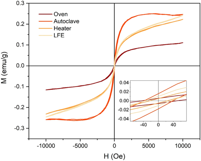
VSM diagram of FGPs to determine the contribution of temperature, pressure, and magnetic field in magnetism. The hysteresis loop of all samples and the zoom part of diagram − 90 < H < 90 (Oe) and − 0.045 < M < 0.045 (emu/g) in the inset.
Full size image
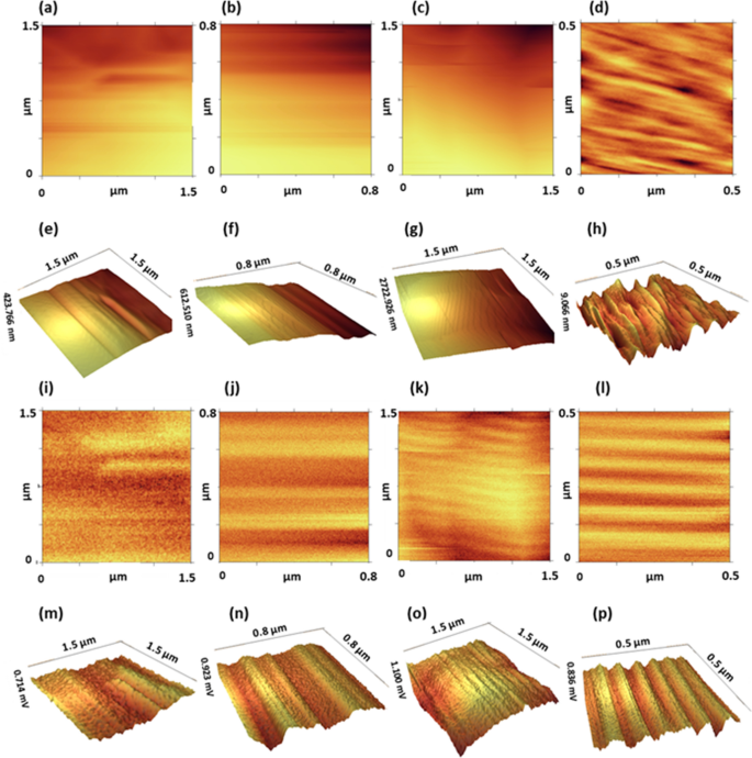
MFM images of all samples in Oven-, Autoclave-, Heater-, and LFE-method (left–right). (a–d) 2D topography images. (e–h) 3D topography images. (i–l) 2D amplitude images. (m–p) 3D amplitude images of FGPs in Oven-, Autoclave-, Heater-, and LFE-method, respectively (left–right).
Full size image
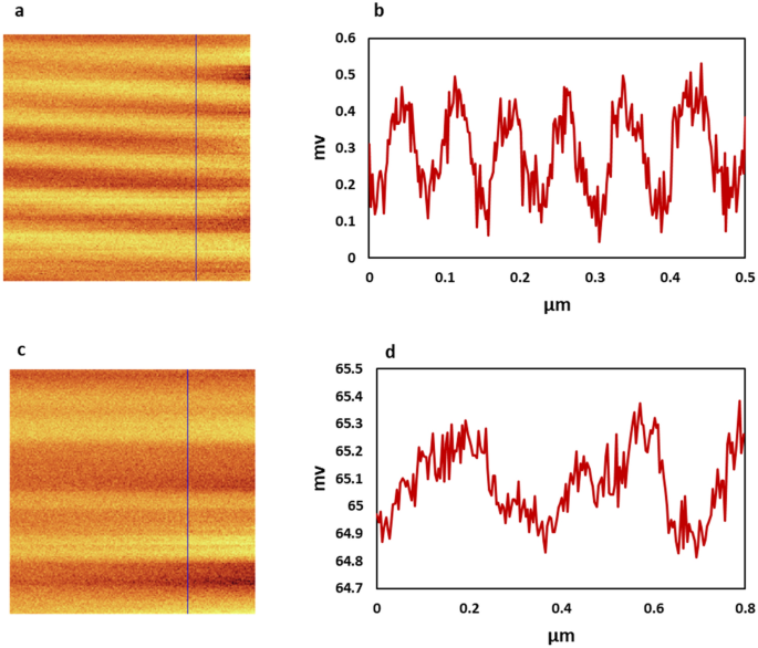
Magnetic domains of LFE- and Autoclave-samples and their domain size. Amplitude images and profile of blue line (a,b) LFE-method. (c,d) Autoclave-method.
Full size image
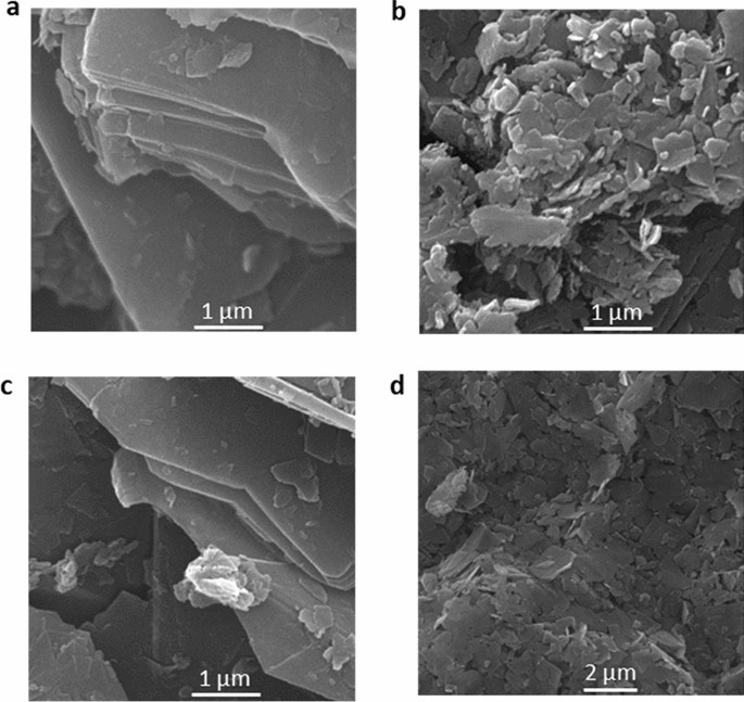
SEM images of FGPs. (a–d) the Oven, Autoclave, Heater, and LFE, respectively. The difference between stacking and aggregation process is obvious in the images. (a,c) Stacking. (b,d) Aggregation.
Full size image
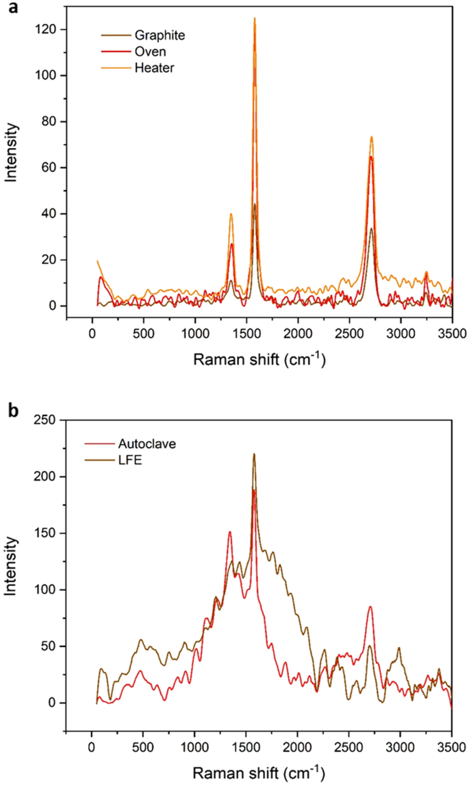
Vibrational modes of FGPs samples in Raman spectra. (a) Raman spectra of Graphite, Oven- , and Heater-method. (b) Raman spectra of Autoclave- and LFE-method.
Full size image
Ferromagnetic graphene
Ferromagnetic behavior of graphene powders is investigated by vibrating sample magnetometer (VSM) and the results are shown in Fig. 2. Due to the natural defects (ID/IG ~ 0.25) and negligible impurities such as Ni, Co, Fe, and Mn, the weak ferromagnetic behavior is observed in pristine graphite (Supplementary Fig. S1 and Table S1). As shown in Fig. 2, the magnetization saturation (Ms) of FGPs is different in the methods. In FGPs, ~ 0.08 emu/g as Ms is generated by temperature in Oven-method, ~ 0.24 emu/g is generated by temperature and pressure in Autoclave-method, and ~ 0.16 emu/g is generated by temperature and the magnetic field in Heater-method. Clearly, the contribution of temperature, pressure, and magnetic field in the magnetization of graphene is ~ 0.08, 0.16, and 0.08 emu/g, respectively. Because of the better comparison in magnetic domains, the 4000 rpm sample of LFE is used in this study (Ms ~ 0.16 is near to other FGPs). Therefore, for comparison of Ms, the Ms of 3000 rpm LFE-sample is reported ~ 0.4 emu/g, indicated the simultaneous effect of all parameters45.
Similar to LFE-method, the slope created in the VSM diagram of Heater-method in high magnetic fields, related to the non-uniformity of particles. In Heater-method, the non-uniform conditions are felt by flakes because of gradual removal of the solution, non-uniform of the magnetic field, and non-uniform heat flow. In LFE-method, the slope created is related to the different behavior of droplets45. Because the temperature and pressure are applied in all directions, all flakes can be felt the same conditions in Oven- and Autoclave-method. The details of the hysteresis loop were summarized in Supplementary Table S2 and are in the inset of Fig. 2.
Magnetic domains
Magnetic force microscopy (MFM) is used to observe the magnetic domains. This technique is similar to atomic force microscopy (AFM), based on cantilever oscillations. The surface of materials is probed by the magnetic tip in different distances. Each line is scanned twice, in one of them, the tip moves near the surface to collect the topography data and in another one the tip moves far from the surface to collect magnetic data56. In Fig. 3, 2D and 3D form of topography and amplitude images for FGPs are presented. Phase images are similar to amplitude, which are presented in Supplementary Fig. S2. All data were collected by a silicon magnetic tip coated by Co and Cr. Because of the unstable small flakes on the powders, moved by the tip, a lot of noises are created and disrupted images. Hence, the disrupted part is cropped that is why the scale of images are different. In the comparison of the topography and amplitude images, the clear magnetic lines are observed in amplitude at flight modes, which indicate parallel magnetic domains. However, the magnetic domains are observed in all samples, LFE- and Autoclave-sample have particular pattern and the grain size of them are ~ 0.1 and 0.4 μm, respectively (Fig. 4).
Raman and IR spectroscopy
Raman and IR spectrum complement each other and show an excellent map of active vibrational modes. By means of these techniques, a lot of information is obtained about the electronic systems and the lattice vibrational modes of graphene at Brillouin Zone (BZ). Raman spectroscopy is widely considered as a key diagnostic tool for symmetric vibrational modes, whereas IR is used for recognizing the asymmetric modes. Although most vibrational modes are active, some of the modes are silent. Generally, in Raman spectroscopy, the laser light is used to excitation and Raman scattering is detected. In addition, the electronic band structures can involve in the resonance process such as double resonance (DR) and triple resonance (TR) Raman process. For example, the phonon modes far from the center of BZ are activated by the DR Raman process. Whereas, at Γ point the phonon is usually activated by first-order Raman process57,58,59,60.
Lattice structure, the lattice vibrations, the electronic systems, and their changes can be investigated by Raman spectroscopy. Therefore, each parameter that affects the electronic systems and phonon modes of graphene can be detected and probed by Raman spectroscopy57. Raman spectra of all FGPs and graphite are shown in Fig. 6. Also, all effective parameters in these Raman spectra such as the number of layers, stacking order, twisting, and also the external perturbation such as strain, magnetic field, and temperature are discussed below. The wavelength of the laser used in this study is 532 nm and its spot size is 0.72 μm. Indeed, the area of the sample is covered by laser light is 0.72 μm, in each measurement. Many flakes can exist in this area which is different at the number of layers, stacking order, twisting, and electronic systems.
Interpretation of the vibrational mode is based on the structural symmetry and group theory. The highest symmetry is D6h, which is belonged to one-layer graphene and graphite, at the Γ point. The irreducible representation of them are ΓGraphene = A2u + B2g + E1u + E2g and ΓGraphite = 2(A2u + B2g + E1u + E2g). Three optical modes in graphene are E2g (Raman active) and B2g (silent). In graphite, nine optical modes exist containing three IR active, five Raman active, and one silent (B2g) modes. IR active modes are a doubly degenerate E1u appear in ~ 1588 cm−1, generated from asymmetric in-plane vibrational mode and one asymmetric out-of-plane mode, A2u, located in ~ 868 cm−1 57,61. In Supplementary Fig. S3, the IR spectrum for all samples is presented and E1u and A2u modes are observed in most samples. Also, these two peaks are too weak in graphite and LFE-sample. For graphite and LFE-sample, E1u peak is located at ~ 1525 cm−1 and in the other samples broadening and redshift of E1u peak is observed.
By increasing the number of layers, the symmetry is reduced and subsequently, the modes are changed. For example, N-layer graphene (NLG) symmetry with the even and odd layers is D3d and D3h at Γ point, respectively. Also, the symmetry information along the Γ–K direction is different and their phonons are activated by DR Raman process. For example, the symmetry of monolayer and NLG (even) at M point is D2h and C2h, respectively58,62. Generally, changes in the electronic system and the lattice structure can create new modes, and even the combination and splitting of some modes can appear the complex modes in the Raman spectrum.
Basically, three characteristic peaks exist in graphene Raman spectra. One of the main peaks in Raman spectra is generated from symmetric in-plane vibrational mode, located in ~ 1580 cm−1. These doubly degenerate, E2g, is called G mode and its position is sensitive to external perturbations, such as defects, doping, strain, and temperature. The two other peaks appear in ~ 2670 and 1200 cm−1, called 2D and D, respectively57.
Ultralow-frequency modes
Ultralow-frequency modes are directly related to interlayer vibrations. In graphite, the out-of-plane and in-plane interlayer vibrations, layer-breathing (LB) and shear (C) modes, are related with B2g (~ 128 cm−1) and E2g (~ 43.5 cm−1) modes, respectively. As another example in AB-2LG, C and LB modes are located at ~ 31 cm−1 (Eg) and ~ 90 cm−1 (A1g), respectively. In addition, C mode in AB-3LG and ABC-3LG are located at ~ 33 cm−1 and ~ 19 cm−1, respectively. Generally, interlayer vibrations depend on twisting, stacking order, and the number of layer57,61,63,64,65,66,67,68. In Fig. 4a, the Raman spectra of graphite, Heater-, and Oven-sample are shown and no special modes are observed between 0 and 1000 cm−1, however, many modes are observed in Fig. 4b for LFE- and Autoclave-sample. These differences are related to the aggregation and stacking process.
D mode
D mode requires defects for activation. This mode is used to characterize defects in graphene. Generally, the ID/IG is used to estimate the amount of defects in graphene flakes57. Only edge defects can be created in the samples, related to the sonication process in the dispersion of graphene. Because of using the same dispersion method in all samples, it is expected that the edge defects are the same and ID/IG are equal (Supplementary Table S3) but in aggregation process the number of edges, exposed to the laser light are more than the stacking. Moreover, the complexity of D mode in Supplementary Fig. S4b related to combination and creation new modes.
G mode
G mode is originated from a first-order Raman scattering process and related to E2g mode at Γ point. In graphene and graphite, G mode is located in ~ 1582 cm−1 and is sensitive to external magnetic fields, strain, and temperature. According to published studies, discrete Landau levels are created in graphene by perpendicular magnetic fields. In addition, the energy and filling factor of Landau levels depend on the strength of the external magnetic field. Electron transition between these levels and resonance process with optical phonons are known as magneto-excitons and magneto phonon resonances, respectively. These are led to new optically modes, detected by Raman spectra. For example, when one-layer graphene is exposed to the perpendicular magnetic field, the symmetry representation of allowed transitions are A1, A2, and E2 which the E2 and E2g (origin of G peak) can interact. Therefore, the position and the shape of the G peak are changed and led to broadening and splitting57,69,70,71,72. Broadening of G mode in Heater-method can be related to the new modes such as E2 (Supplementary Fig. S4c).
Changing the interatomic distance in crystal lattice under stain and stress lead to manipulating electronic systems. Recently, the strain effect on electronic systems is considered and remarkable results such as shifting the Dirac cones, opening band gap, shifting and splitting Raman modes, and inducing strong pseudo-magnetic field is reported. As an example, in graphene, shifting the vibrational frequency and splitting the G mode (G+ and G−) is observed under stress. In addition, the G mode are sensitive to temperature42,57,73,74,75,76,77,78,79,80.
2D mode
2D (~ 2700 cm−1) is activated by the resonance process. The component of the 2D peak dependent on electronic bands and laser wavelengths. Here, the laser wavelength is the same in all measurements. Due to several electronic bands are in multilayer graphene, the many 2D components can be expected. Because of these features, the 2D peak is used to determine the number of layers. In addition, the stacking order also can be strongly effected on electronic bands and change the spectral profile of the 2D peak. Therefore, the complexity of 2D LFE-sample and Autoclave-sample compared to other samples can be related to more manipulation of electronic systems (Fig. 6b). In addition, 2D peak is sensitive to temperature and strain. Moreover, in the presence of strain, deformation of Dirac cones is led to splitting 2D modes into 2D+, and 2D−57,66,76,81,82,83,84.
Source www.nature.com