Neural Bar Impulse: Research and Implementation

The Research

Our goal was to forecast the next price bar. But how? Do we need to know all four price points — open, high, low, close? We concluded that this is not necessary. If we are going to trade within the future bar, it is important to know in which direction it is more preferable to open positions and at what distance from the opening price to set take-profit or stop-loss levels. We need to know which direction the price within the future bar is likely to trend towards: whether it will mostly break through the upper or lower extremes.

So, we focused on the price movement characteristics within the bar. We attempted to capture this abstract concept in a mathematical formula:

I_b = (High_b - Open_b) - (Open_b - Low_b)

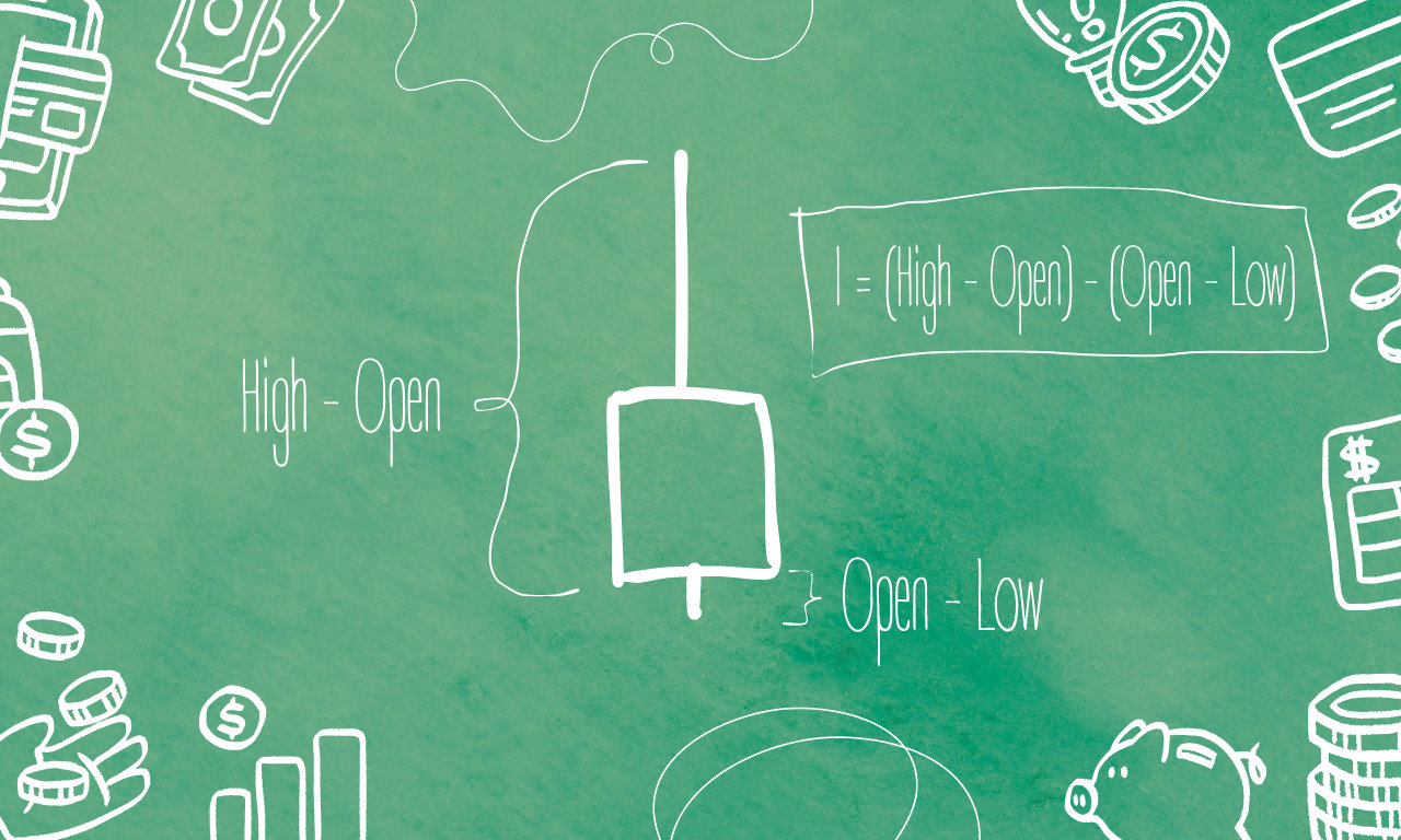
We named this value the “bar impulse”. It demonstrates the strength and direction of price movement within the bar. Essentially, it is the difference between two ranges: from the bar's high to the opening price and from the opening price to the bar's low. This metric is optimal for us because it is both simple and informative. Using four price levels (open, high, low, close) can introduce additional noise and complexity in analysis. The bar impulse focuses on the most significant changes (differences between ranges), simplifying the model and reducing the amount of required information.

If the bar impulse value is positive, it indicates that the price tends to move upwards from the opening price, while a negative value indicates a tendency to move downwards. This helps traders better understand the likely direction of price movement within the future bar. This is the quantity we are trying to predict using artificial intelligence.

The next important step in our research was the development of a neural network and the collection of data for its training. To address the task, we used a recurrent neural network and built a model based on the Long Short-Term Memory (LSTM) architecture, consisting of several layers designed for analyzing sequential data with long-term dependencies.

These LSTM layers allow the model to account for information about past financial market states and use it to make decisions about future states. I will not delve into technical details, but I will note that in designing the neural network, we aimed to find the optimal balance between its complexity and alignment with expected results.

But why did we choose this type of neural network? Financial data, such as currency pair prices, represent time series where the current state strongly depends on previous states. RNNs, especially LSTMs, are specifically designed to handle such sequential data and account for long-term dependencies. Unlike traditional RNNs, which can suffer from the vanishing gradient problem when training on long sequences, LSTMs have a special architecture that includes "memory cells" and mechanisms for managing the flow of information. This allows them to effectively retain and use information about earlier states in the sequence.

Standard RNNs often face the vanishing gradient problem, where gradients become too small when passing information through many time steps. LSTM addresses this issue by using specialized cells and mechanisms for forgetting and updating information, which allows it to effectively handle long-term dependencies. Financial data often contains noise and short-term fluctuations, which can complicate model training. LSTM’s ability to focus on the most significant data and ignore less important elements helps improve robustness to noise and increase prediction accuracy.

We fed the neural network with data representing time series, where each element contains information about price bars. Typically, this includes the open, high, low, and close prices. The data was presented as sequences of time series, where each time step contains a set of values for one bar. For example, a sequence might look like this: [Open_t, High_t, Low_t, Close_t], where "t" is the current time step.

To improve training efficiency, the data is often normalized or standardized. For example, min-max normalization can be used to scale all values to the range from 0 to 1.

For training the LSTM, it was also important to prepare the data as windows of sequences. If you use a window of length N, it means that for each time step, the input sequence will contain N previous bars. For example, if the window length is 10, then to predict the next bar, you will use data from the 10 previous bars. The input array for the LSTM would look like this:

[
Open_{t-10} & High_{t-10} & Low_{t-10} & Close_{t-10}
Open_{t-9} & High_{t-9} & Low_{t-9} & Close_{t-9}
Open_{t-8} & High_{t-8} & Low_{t-8} & Close_{t-8}
...
Open_{t-2} & High_{t-2} & Low_{t-2} & Close_{t-2}
Open_{t-1} & High_{t-1} & Low_{t-1} & Close_{t-1}
]

The model's output is the value of the bar impulse for the next time step. In other words, the model predicts how strongly the price will move up or down from the opening price in the next bar. If the model predicts the bar impulse for the next time step, the output array might look like:

[I_{t+1}], where I_{t+1} is the predicted value of the bar impulse for the next bar.

Since the bar impulse is a continuous value, the task is a regression problem. Therefore, the neural network’s output layer has a single neuron that provides the continuous impulse value.

We fed the neural network with historical data on major currency pairs in the Forex market, starting from 2001 to the present day. Millions of bars were processed by the neural network for evaluation, training, and testing of this mathematical model. This was a complex and technically demanding process. Let us present to you some modest aspects of visualizing this action.

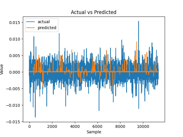
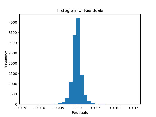
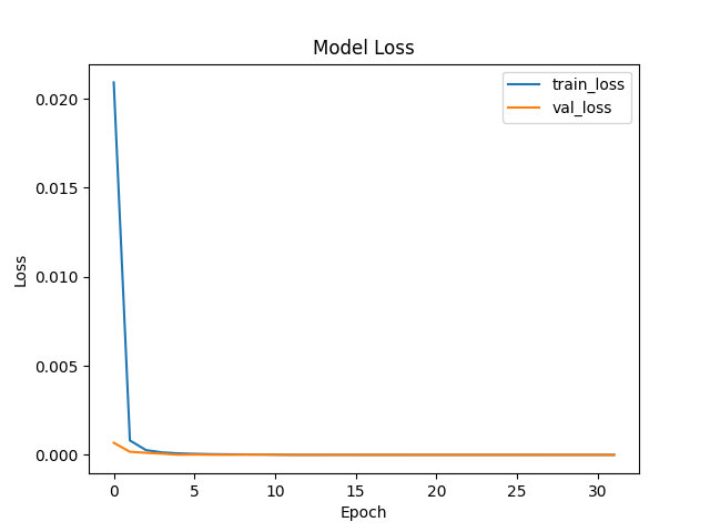
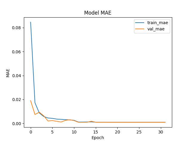
The histogram “Actual vs Predicted” is a graphical representation comparing the actual and predicted values of the target variable in a machine learning model. The trained model was tested on 10 thousand bars. Here we can observe the spread of bar impulse values. “Histogram of Residuals” allows us to assess how well the model performs in predicting the response variable. If the residuals are evenly distributed around zero and follow a normal distribution, it may indicate that the model fits the data well and does not have systematic errors. The “Model Loss” and “Model MAE” plots reflect the standard and mean absolute errors of the model at each stage of training among all 32 epochs. The lower their values, the better the model performs in predicting the variable of interest.

After completing all the aforementioned procedures, we have achieved a refined outcome: a trained neural network capable of analyzing historical quotes of financial instruments and predicting the impulse of the next bar.

The Implementation

Through careful data analysis and visualization methods, we evaluated the effectiveness of the model in predicting market behavior. We intended to use the obtained data to develop practical trading products. These products include a trading indicator and bot based on predicting the impulse of the next price bar using neural networks. Our goal is to provide traders with tools that will help them make more informed decisions and increase profitability in financial markets.

The first step in bringing our idea to life was to create a trading indicator using the MQL5 programming language. This language is constantly evolving, absorbing increasingly high-tech elements, including the ability to work with neural networks and other artificial intelligence algorithms. It enabled us to fully model the functionality of our indicator, which we named the “Neural Bar Impulse”.

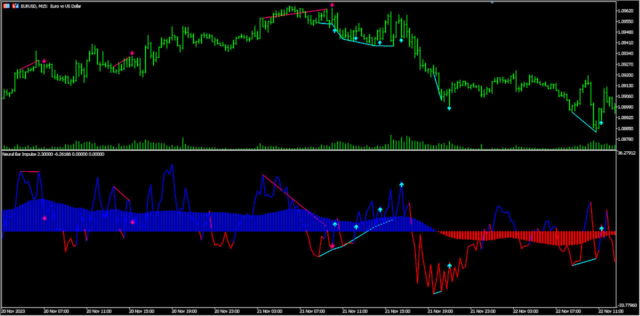
The image above is divided into two parts. In the upper part, there is a price chart of the financial instrument, and in the lower part, there is our created indicator. It consists of an oscillating two-color line, representing the values of the indicator obtained from the trained neural network. Based on this data, the indicator also constructs a moving average, displayed on the chart as a two-color histogram. Additionally, you can see two two-color lines, converging and diverging from each other, crossing the price and indicator extremes – these are convergence and divergence lines. I will explain more about these lines later. And the final element of the indicator is two-color arrows pointing up or down, depending on the type of indicator signal.

Initially, our indicator was simply an oscillating line forecasting the impulse of the next bar. However, during testing, we noticed too much noise in its readings. After brainstorming and exploring various options, we settled on using divergence/convergence. We concluded that this would be the most optimal approach for filtering out overly frequent noisy indicator signals and for scaling the analysis beyond just a single bar.

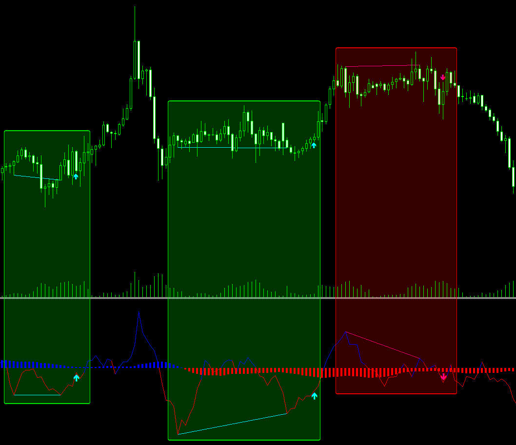
In the image above, I have highlighted specific zones where we can observe crucial patterns necessary for analysis and decision-making regarding the signal situation. Both the price and the indicator exhibit visually and programmatically identifiable extremes, or, in simpler terms, “peaks” and “valleys”. Based on these local maxima and minima, the indicator draws lines connecting them and examines whether there are any differences between them. These differences may manifest in the form of divergences or convergences, meaning moments when the price moves up or down at extremes while the indicator line descends or ascends in the opposite direction. When such a pattern completes its formation, the indicator displays an arrow in the corresponding direction. These arrows simultaneously serve as signals for traders, indicating that it is time to open a position in a particular direction.

What is the advantage of such analysis? How does this method complement the neural network forecasts? Let’s take a look at the latest picture again. Does the actual bar impulse always coincide with the forecasted one? No, because there are no 100% accurate forecasts, and deviations always exist. However, we can protect ourselves from these inaccuracies. Instead of focusing on individual cases, we can analyze trends. If the indicator line consistently rises or falls with each subsequent bar, we can speak of a certain trend in forecasting. Similarly, we can assess the increasing or decreasing extremes of the indicator. What do we see on the chart? The price continues to decline, its extremes are decreasing, indicating a downtrend. However, the extremes of the indicator are increasing. This suggests that there is a trend in the neural network forecasts that is opposite to the price movement. This serves as a signal for a reversal in the price trend. Essentially, what have we done? We have reformatted the forecasting of each bar’s impulse into forecasting the trend of bar impulses, or more precisely, forecasting reversals of these trends.

In continuation of our research implementation, based on the “Neural Bar Impulse” indicator, we have developed a trading robot – a software application capable of automating trades on financial markets without direct human involvement. The algorithm of the bot encompasses calculations based on the indicator, including interaction with the trained neural network, as well as a functional component responsible for executing trades and monitoring the market. This comprehensive approach enables traders to maintain objectivity in decision-making, minimize the influence of emotions, avoid human errors, and analyze extensive volumes of historical data.

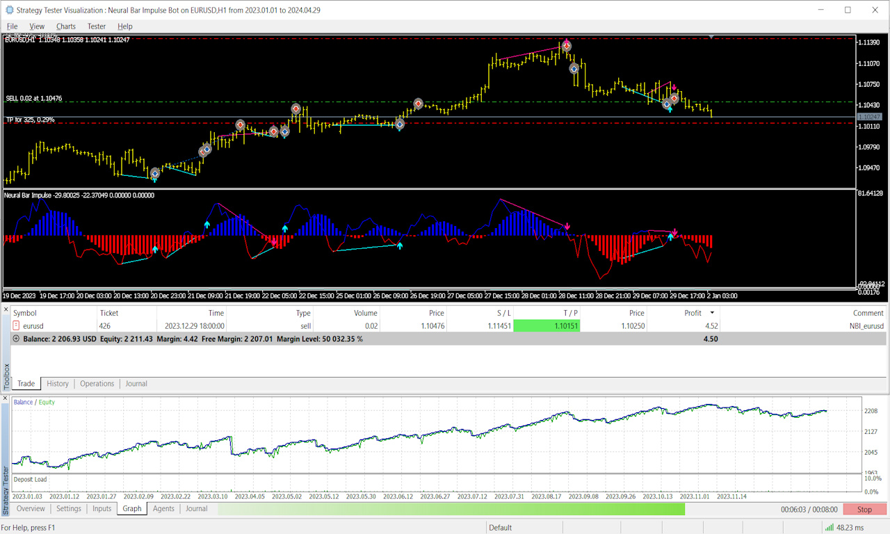
Before allowing a trading bot to conduct operations on a real account, we undergo meticulous testing and optimization on historical data. It’s not just about analyzing dry statistical metrics, but also visually assessing the bot’s performance. The image above captures one such process: the bot, guided by indicator signals, successfully initiated a sell position, and the price confidently moved downward, reaching the take-profit level. The lower part of the terminal displays the balance and equity curve, enabling us to analyze the bot’s behavior under various market conditions. Visualization aids not only in testing, but also in enhancing the functionality of trading bots and advancing the original concept.

As algorithmic traders, our mission extends far beyond simply bringing trading ideas to life. We strive for their continual development, allowing them to evolve much like the vast universe, where no single formula can encompass all aspects. Similarly, in trading, relying on a single trading idea to explain the full spectrum of market phenomena is impractical. Financial markets are complex systems of interaction, demanding thoughtful and original solutions. The rapidly changing environment requires traders to remain flexible in strategy creation and disciplined in execution. This is where trading indicators and bots come into play, helping to provide the flexibility and reliability needed to implement strategies. Our example of research and implementation only hints at the comprehensive approach required to overcome the challenges of the financial market.