Linear algebra for game developers: Part II
Games Development
Basis Vectors
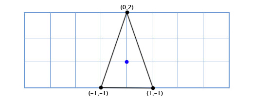
Let's say we're making an Asteroids game on really old hardware, and we want to have a simple 2D space ship that can rotate freely. The ship model looks like this:
So how do we draw it when the player rotates by an arbitrary amount, like 49 degrees counter-clockwise? Well, trigonometry we can create a function for 2D rotation that inputs a point and an angle, and outputs a rotated point:
   vec2 rotate(vec2 point, float angle){
           vec2 rotated_point;
           rotated_point.x = point.x * cos(angle) - point.y * sin(angle);
           rotated_point.y = point.x * sin(angle) + point.y * cos(angle);
           return rotated_point;
   }
Applying this to our three points gives us the following shape:
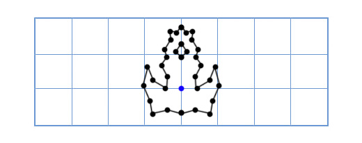
Cosine and sine operations are pretty slow, but we're only doing them on three points, so it can smoothly on our old hardware. But now we decide to upgrade the ship to look like this:
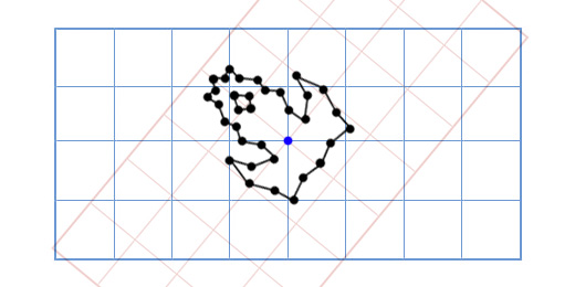
Now our old method is too slow! We don't have enough sine and cosine operations to rotate this many points. There are many ways to solve this problem, but an elegant solution comes to us like this: "What if instead of rotating each point in the model, we just rotate the model's x and y axes instead?"
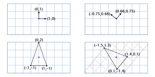
How does this work? Well, let's look at what coordinates mean. When we talk about the the point (3,2), we are saying that its position is three times the x-axis plus two times the y-axis. The default axes are (1,0) for the x-axis and (0,1) for the y-axis, so we get the position 3(1,0) + 2(0,1). But the axes don't have to be (1,0) and (0,1). If we rotate these axes, then we can rotate every point at the same time.
To get the rotated x and y axes we just use the trigonometric function above. For example, if we are rotating by 49 degrees, then we get the new x-axis by rotating (1,0) by 49 degrees and we get the y-axis by rotating (0,1) by 49 degrees. Our new x-axis is (0.66, 0.75), and our new y-axis is (-0.75, 0.66). We can do this by hand for our 3-point model to prove that it works:
The top point is (0,2), which means its new position is zero times the rotated x-axis plus twice the rotated y-axis.
0*(0.66,0.75) + 2*(-0.75, 0.66) = (-1.5, 1.3)
The bottom-left point is (-1,-1), which means its new position is negative one times the rotated x-axis plus negative one times the rotated y-axis.
-1*(0.66,0.75) + -1*(-0.75, 0.66) = (0.1, -1.4)
The bottom-right point is (1,-1), which means its new position is one times the rotated x-axis plus negative one times the rotated y-axis.
1*(0.66,0.75) + -1*(-0.75, 0.66) = (1.4, 0.1)
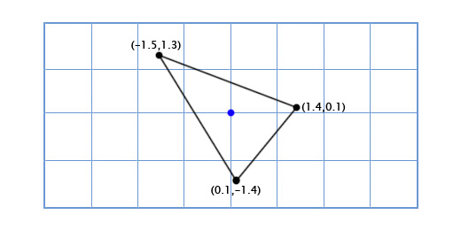
What we are doing here is using the ship coordinates as if they exist in a separate coordinate system with rotated axes (or 'basis vectors'). This is useful in this case because it separates the cost of manipulating the orientation of the ship from the cost of applying the orientation to the model points.
Whenever you have modified the basis vectors (1,0) and (0,1) to (a,b) and (c,d), then the modified point (x,y) can be found using this expression:
x(a,b) + y(c,d)
Normally the basis vectors are (1,0) and (0,1) so you just get x(1,0) + y(0,1) = (x,y), and you don't have to bother with this. However, it's important to remember that you can use other bases (plural of basis) as well.
Matrices
Matrices are like 2-dimensional vectors. For example, a typical 2x2 matrix might look like this:
   [a c
    b d]
When you multiply a matrix by a vector, you sum the dot product of each row of the matrix with the vector. For example, if we multiply the above matrix with the vector (x,y), we get:(a,c)•(x,y) + (b,d)•(x,y)
Written another way, this is:
x(a,b) + y(c,d)
Look familiar? This is the exact same expression that we use when changing the basis vectors! This means that multiplying a 2x2 matrix with a 2D vector is the same thing as changing its basis vectors. For example, if we plug the standard basis vectors (1,0) and (0,1) into the matrix columns, we get:
[1 0
 0 1]
This is the identity matrix, which has no effect, as we would expect from the neutral basis vectors we chose. If we plug in our 49-degree rotation bases, we get:[0.66 -0.75
 0.75  0.66]
This matrix will rotate any 2D vector counter-clockwise by 49 degrees. We could write our asteroids program with a lot more elegance by using matrices like this. For example, our ship-rotation function could look like this:
void RotateShip(float degrees){
        Matrix2x2 R = GetRotationMatrix(degrees);
        for(int i=0; i<num_points; ++i){
                rotated_point[i] = R * point[i];
        }
}
However, it would be even more elegant if we could include translation (movement through space) in the matrix as well. Then we would have a single data structure that can elegantly store and apply the orientation and position of each object. Fortunately, there is a way to do this, even though it's a bit of an ugly hack. If we want to translate by a vector (e,f), we can just tack it onto our change-of-basis matrix like this:[a c e
 b d f
 0 0 1]
And then we add an extra [1] to the end of each position vector like this:[x y 1]
Now when we multiply them together we get:(a,c,e)•(x,y,1) + (b,d,f)•(x,y,1) + (0,0,1)•(x,y,1)
Which can essentially be rewritten:x(a,b) + y(c,d) + (e,f)
So now we have the entire transformation in a single matrix! This is important for many reasons aside from just elegant code, because now we can use all of the standard matrix manipulation tools on it. For example, we can multiply matrices together to add their effects, or we can invert a matrix to give it the exact opposite transformation.3D Matrices
Matrices in 3D work just like they do in 2D -- I just used 2D examples in this post because they are easier to convey with a 2D screen. You just define three columns for the basis vectors instead of two. If the basis vectors are (a,b,c), (d,e,f) and (g,h,i) then your matrix should be:[a d g
 b e h
 c f i]
If you need translation (j,k,l), then you add the extra column and row like before:[a d g j
 b e h k
 c f i l
 0 0 0 1]
And add an extra [1] onto the vectors like this:[x y z 1]
2D Rotation
Since there is only one possible axis of rotation (the axis going into the screen), the only information we need is the angle. I mentioned last time that using trigonometry we can create a 2D rotation function like this:
vec2 rotate(vec2 point, float angle){
        vec2 rotated_point;
        rotated_point.x = point.x * cos(angle) - point.y * sin(angle);
        rotated_point.y = point.x * sin(angle) + point.y * cos(angle);
        return rotated_point;
}
This is more elegantly expressed in matrix form. To find the matrix version, we can apply the function to the axes (1,0) and (0,1) for angle θ, and then plug the new axes into the columns of our matrix. Let's start with the x axis: (1,0). If we plug it into our function we get:
(1*cos(θ) - 0*sin(θ), 1*sin(θ) + 0*cos(θ)) = (cos(θ), sin(θ))
Next, we plug in the y axis: (0,1). This gives us:
(0*cos(θ) - 1*sin(θ), 0*sin(θ) + 1*cos(θ)) = (-sin(θ), cos(θ))
Plugging these new axes into the columns of a matrix gives us our 2D rotation matrix:
[cos(θ) -sin(θ)
 sin(θ)  cos(θ)]
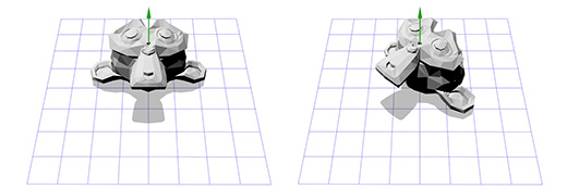
Let's apply this matrix to Suzanne, the Blender monkey, with θ = 45 degrees clockwise.
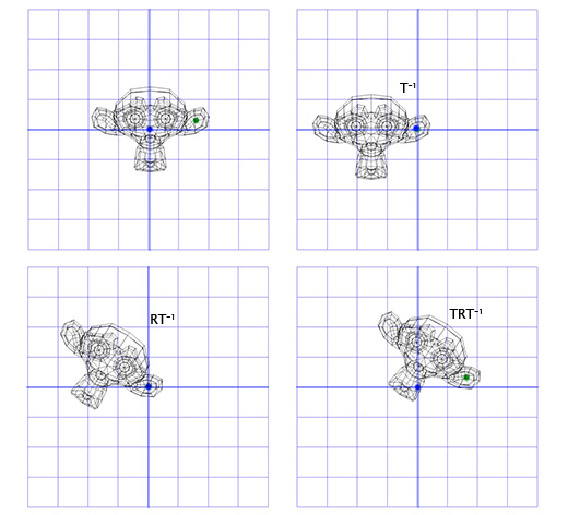
It works! But what if we want to rotate around a point that is not (0,0)? For example, maybe we want the monkey to rotate around a point on its ear, like this:
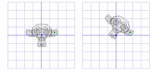
To do this, we can start by making a translation matrix T that moves from the origin to the ear pivot point, and a rotation matrix R that rotates around the origin. Now, to rotate around the ear pivot point, we can first move the ear pivot point to the origin with the inverse of T, written T-1. Then we just rotate around the origin using R, and then apply T to move the pivot point back to its original position. Here is an illustration of each step:
This is an important pattern that we will use again later -- putting the rotation within two opposite transformations lets us do the rotation in a different 'space', which is very useful. Now, let's look at 3D rotation.
3D Rotation
Rotation about the Z axis works just like it did in 2D. We just have to adapt our old matrix by adding an extra column and row:
[cos(θ) -sin(θ) 0
 sin(θ)  cos(θ) 0
 0       0      1]
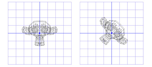
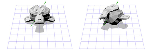
Let's apply this matrix to the 3D version of Suzanne, with θ = 45 degrees clockwise.
Pretty much the same so far! It's pretty limiting to just rotate around the z-axis though -- maybe we want to rotate around any axis we want.
Axis-angle rotations
The axis-angle rotation format represents rotations like this: (axis, angle). Simple enough! This format is very useful, and is the starting point of many of the rotations I work with. But how do we actually apply an axis-angle rotation? Let's say we have a weird axis like this one:
That seems tricky -- but we already have the tools to do it. We know how to rotate around the z-axis, and we know how to rotate in different spaces. So, we just have to create a new space where this axis is the z-axis! But if this axis is the z-axis, what are the x and y axes? That's what we have to construct now.
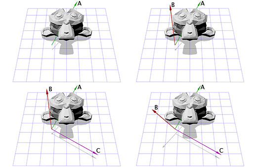
To create the x and y axes, we just have to pick two vectors that are perpendicular to the new z-axis, and perpendicular to each other. Fortunately for us, we talked about the 'cross product' in part two, which inputs two vectors and outputs a perpendicular one. We only have one vector so far, the rotation axis -- let's call it A. Now we can just pick a vector B at random, as long as it's not in the same direction as A. Let's pick (0,0,1) for convenience.
Now that we have the rotation axis A and our random vector B, we can get the normalized cross product, C, which is perpendicular to both other vectors. Now we can make B perpendicular by setting it to the cross product of A and C, and we have our axes!
This sounds complicated when put in words, but it's actually really simple in code or in images. Here's how it would look in code:
B = (0,0,1);
   C = cross(A,B);
   B = cross(C,A);
Here is an illustration of each step :
Now that we have our new axes, we can create a matrix M by plugging in each axis into a column. We have to make sure that vector A is in the third column in order to make it the new z-axis:
[B0 C0 A0
 B1 C1 A1
 B2 C2 A2]
Now it's like what we did for the ear pivot in 2D. We can apply the inverse of M to move into our new coordinate space, then apply rotation R to rotate around the z axis, and then apply M to move back into our usual space.
If that made sense to you, then congratulations, you can rotate around any axis! After all that work, we can just create a matrix T = M-1RM and use it as many times as we like without any further effort. There are more efficient ways to convert axis-angle rotations to matrix rotations, but this way covers a lot of what we've been talking about.
Axis-angle rotations are perhaps the most intuitive rotation format. They are also the easiest to invert (switch the sign of the angle), and the easiest to interpolate (just interpolate the angle). However, they have a serious limitation in that they cannot accumulate. That is, you can't combine two axis-angle rotations into a third. Axis-angle rotations are a good starting place, but they have to be turned into something else to be used for anything complicated.
Euler angles
Euler angles (pronounced 'oyler') are another common rotation format, consisting of three nested rotations around the x, y and z axes. They are probably most familiar to you from the standard first-person or third-person game cameras.
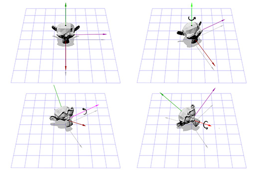
Let's say you're in an FPS game and you rotate 30 degrees left, and then look 40 degrees up. Finally, someone shoots you, and the impact effect rolls the camera on its axis 45 degrees. Here's an illustration of this ZYX euler angle (30, 40, 45)
Euler angles are convenient because they're intuitive and easy to control. However, they do have two drawbacks which limit their use:
First, it's possible to reach a situation called 'gimbal lock'. Imagine you are in the first-person shooter we just described, where you can look left, right, up and down, or roll the camera on its axis. Now imagine you are looking straight up. In this situation, looking left or right is the same thing as rolling the camera -- all we can do is roll the camera or look down! As you can imagine, this limitation makes Euler angles impractical for flight simulators.
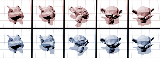
Second, interpolating between two Euler angle rotations does not give the shortest path between them. For example, here are two interpolations between the same rotations. The first is using Euler angle interpolation, and the second is using spherical linear interpolation (SLERP) to find the shortest path.
So what is good for interpolating rotations? Would matrices work better?
Matrix rotations
As we've discussed, rotation matrices just store the three axes. This means that interpolating between two matrices just linearly interpolates each axis. This does result in an efficient path, but also introduces other problems. For example, here are two rotations and an interpolated half rotation:
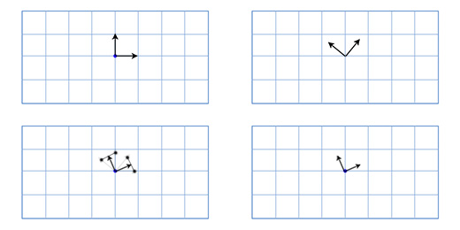
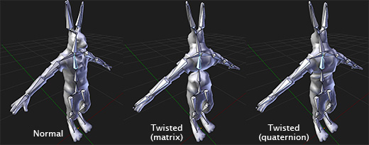
As you can see, the interpolated rotation is significantly smaller than either of the source rotations, and the two axes are no longer perfectly perpendicular. This makes sense if you think about it -- if you average the position of any two points on a sphere, then you will end up closer to the center. This problem causes a trademark 'candy wrapper' effect when used for skeletal animation. Here's an Overgrowth rabbit demonstrating this effect:
Matrix rotations are very useful in that they can accumulate without any problems like gimbal lock, and can most efficiently be applied to points. This is why they are used natively on graphics cards -- for any kind of 3D graphics, the matrix format is always the end goal.
However, as we've seen, they do not interpolate well, and they are not very intuitive to create in many cases.
Well, there's only one major rotation format left. Last but not least, we have:
Quaternions
So what are quaternions? The quick and dirty answer is they are an alternate form of axis-angle rotations that lives in 'rotation space'. Like matrices, they can accumulate -- that is, you can chain them together indefinitely without any problems like gimbal lock. However, unlike matrices, they can smoothly interpolate from one orientation to another.
Are quaternions just better than all the other rotation formats? So far, they seem to combine all of their strengths. Unfortunately, they have two major weaknesses that ensure that they are only useful as intermediate rotations. First, they have no easy mapping to 3D space, so you will always create rotations in a more user-friendly format and convert it over. Second, they cannot efficiently rotate points, so you have to convert them to matrices in order to rotate significant numbers of points.
This means you will likely never start or end a series of rotations with a quaternion, but they can do intermediate processing more efficiently than any other format.
The internal workings of quaternions are not really intuitive or interesting to me, and probably won't be for you either if you're not a mathematician, so I advise finding libraries or functions online that wrap quaternions in a way that makes them easy to use. The Bullet or Blender math libraries could be a good place to start, and there are many others on the Internet.
Thanks for reading, are you still in?
If you enjoyed this article, it would be cool if you press like, or write something to me, it will make me to post more often and more cooler content ;)
Further Reading:
How to launch a side project in 10 days
How to Actually Finish Your First Game?
Top 7 Soft Skills for Developers