DreamGaussian: Generative Gaussian Splatting for Efficient 3D Content Creation
https://t.me/reading_ai, @AfeliaN🗂️ Project Page
📄 Paper
📎 GitHub
🗓 Date: 28 Sep 2023
Main idea

Motivation: existing models for text→3D tasks vis SDS loss have been widely developed recently, But these methods suffer from slow per-sample optimization or may lose quality (like in ATT3D).
Solution: Gaussian Splatting model! Progressive densification of 3D Gaussians converges significantly faster than NeRFs. To further enhance the texture quality and facilitate downstream applications, the authors introduced an efficient algorithm to convert 3D Gaussians into textured meshes and apply a fine-tuning stage to refine the details.
Pipeline

Firstly, a 3D Gaussian splatting model was adapted into a generation task through SDS. Specifically, the location of each Gaussian can be described with a center (x in R^3), scaling factors and a rotation quaternion q. Additionally, an opacity alpha and color feature c are stored for volumetric rendering.
Spherical harmonics are disabled since we only want to model simple diffuse color. To render a set of 3D Gaussians, they need to be projected into the image plane as 2D Gaussians. Volumetric rendering is then performed for each pixel in front-to-back depth order to evaluate the final color and alpha.
The 3D Gaussians are initialized with random positions sampled inside a sphere, with unit scaling and no rotation. These 3D Gaussians are periodically densified during optimization. The authors start from fewer Gaussians but densify it more frequently to align with the generation progress. SDS loss is used for optimization.
In case of image-to-3D the authors adopt Zero-1-to-3 XL as the 2D diffusion prior.

Mesh extraction
To improve the results from this pipeline step (as they may be quite blurry) - the authors suggest additional mesh optimization.
Since the spatial density is described by a large number of 3D Gaussians, bruteforce querying of a dense 3D density grid can be slow and inefficient. It’s also unclear how to extract the appearance in 3D, as the color blending is only defined with projected 2D Gaussians.
Density Query
To extract the mesh geometry, a dense density grid is needed to apply the Marching Cubes.
- 3D space (-1,1)^3 is divided into 16^3 blocks
- Then the Gaussians whose centers are located outside each local block are culled.
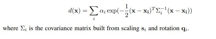
- Then the authors query a 8^3 dense grid inside each block, which leads to a final 1283 dense grid. For each query at grid position x, the authors sum up the weighted opacity of each remaining 3D Gaussian:
Color Back-projection
Firstly the authors unwrap the mesh’s UV coordinates and initialize an empty texture image.
Then 8 azimuths and 3 elevations, plus the top and bottom views were chosen to render the corresponding RGB image. Each pixel from these RGB images can be back-projected to the texture image based on the UV coordinate. Additionally the pixels with a small camera space z-direction normal were excluded to avoid unstable projection at mesh boundaries. This back-projected texture image serves as an initialization for the next mesh texture fine-tuning stage.
UV-Space Texture Refinement
Due to the ambiguity of SDS optimization, the meshes extracted from 3D Gaussians usually possess blurry textures. To solve this problem a second stage to refine texture is proposed. However, fine-tuning the UV-space directly with SDS loss often leads to artifacts due to the mipmap texture sampling technique used in differentiable rasterization.
With ambiguous guidance like SDS, the gradient propagated to each mipmap level results in over-saturated color blocks.
Rather than using SDS loss the authors propose another approach.
First of all, we can render a blurry coarse image from an arbitrary camera view p. Then the image is perturbed with random noise and then denoised using the 2D diffusion prior to obtaining refined images.

This refined image is then used to optimize the texture through a pixel-wise MSE loss:

Implementation detailes
Training process: 500 steps for 1-st stage and 50 for the second.
Resolution: The rendering resolution is increased from 64 to 512 for Gaussian splatting, and randomly sampled from 128 to 1024 for mesh.
Models: Gaussian Splatting Model
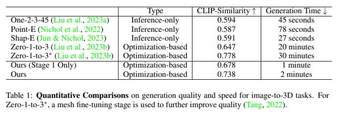
Compared with: DreamFusion, Shape-E, Point-E, One-2-3-45, Zero-1-to-3


Pros and cons
- Pros: much faster and has quite good quality
- Limitations: still the multi-face Janus problem and baked lightning
Results