Building a Search Engine with BERT and TensorFlow
https://t.me/JuicyDataAuthor: https://towardsdatascience.com/@gaphex
In this experiment, we use a pre-trained BERT model checkpoint to build a general-purpose text feature extractor, which we apply to the task of nearest neighbour search.
Feature extractors based on deep Neural Probabilistic Language Models such as BERT may extract features that are relevant for a wide array of downstream NLP tasks. For that reason, they are sometimes referred to as Natural Language Understanding (NLU) modules.
These features may also be utilized for computing the similarity between text samples, which is useful for instance-based learning algorithms (e.g. K-NN). To illustrate this, we will build a nearest neighbour search engine for text, using BERT for feature extraction.
The plan for this experiment is:
- getting the pre-trained BERT model checkpoint
- extracting a sub-graph optimized for inference
- creating a feature extractor with tf.Estimator
- exploring vector space with T-SNE and Embedding Projector
- implementing a nearest neighbour search engine
- accelerating search queries with math
- example: building a movie recommendation system
Questions and Answers
What is in this guide?
This guide contains implementations of two things: a BERT text feature extractor and a nearest neighbour search engine.
Who is this guide for?
This guide should be useful for researchers interested in using BERT for natural language understanding tasks. It may also serve as a worked example of interfacing with tf.Estimator API.
What does it take?
For a reader familiar with TensorFlow it should take around 30 minutes to finish this guide.
Show me the code.
The code for this experiment is available in Colab here. Also, check out the repository I set up for my BERT experiments: it contains bonus stuff!
Now, let’s start.
Step 1: getting the pre-trained model
We start with a pre-trained BERT checkpoint. For demonstration purposes, I will be using the uncased English model pre-trained by Google engineers. To train a model for a different language, check out my other guide.
For configuring and optimizing the graph for inference we will make use of the awesome bert-as-a-service repository. This repository allows for serving BERT models for remote clients over TCP.
Having a remote BERT-server is beneficial in multi-host environments. However, in this part of the experiment we will focus on creating a local
(in-process) feature extractor. This is useful if one wishes to avoid additional latency and potential failure modes introduced by a client-server architecture.
Now, let us download the model and install the package.
!wget https://storage.googleapis.com/bert_models/2019_05_30/wwm_uncased_L-24_H-1024_A-16.zip
!unzip wwm_uncased_L-24_H-1024_A-16.zip
!pip install bert-serving-server --no-deps
Step 2: optimizing the inference graph
Normally, to modify the model graph we would have to do some low-level TensorFlow programming. However, thanks to bert-as-a-service, we can configure the inference graph using a simple CLI interface.
import os
import tensorflow as tf

from bert_serving.server.graph import optimize_graph
from bert_serving.server.helper import get_args_parser


MODEL_DIR = '/content/wwm_uncased_L-24_H-1024_A-16/' #@param {type:"string"}
GRAPH_DIR = '/content/graph/' #@param {type:"string"}
GRAPH_OUT = 'extractor.pbtxt' #@param {type:"string"}
GPU_MFRAC = 0.2 #@param {type:"string"}

POOL_STRAT = 'REDUCE_MEAN' #@param {type:"string"}
POOL_LAYER = "-2" #@param {type:"string"}
SEQ_LEN = "64" #@param {type:"string"}

tf.gfile.MkDir(GRAPH_DIR)

parser = get_args_parser()
carg = parser.parse_args(args=['-model_dir', MODEL_DIR,
                               "-graph_tmp_dir", GRAPH_DIR,
                               '-max_seq_len', str(SEQ_LEN),
                               '-pooling_layer', str(POOL_LAYER),
                               '-pooling_strategy', POOL_STRAT,
                               '-gpu_memory_fraction', str(GPU_MFRAC)])

tmpfi_name, config = optimize_graph(carg)
graph_fout = os.path.join(GRAPH_DIR, GRAPH_OUT)

tf.gfile.Rename(
    tmpfi_name,
    graph_fout,
    overwrite=True
)
print("Serialized graph to {}".format(graph_fout))
There are a couple of parameters there to look out for.
For each text sample, BERT encoding layers output a tensor of shape [sequence_len, encoder_dim] with one vector per token. We need to apply some sort of pooling if we are to obtain a fixed representation.
POOL_STRAT parameter defines the pooling strategy applied to the encoder layer number POOL_LAYER. The default value ‘REDUCE_MEAN’ averages the vectors for all tokens in a sequence. This strategy works best for most sentence-level tasks when the model is not fine-tuned. Another option is NONE, in which case no pooling is applied at all. This is useful for word-level tasks such as Named Entity Recognition or POS tagging. For a detailed discussion of these options check out the Han Xiao’s blog post.
SEQ_LEN affects the maximum length of sequences processed by the model. Smaller values will increase the model inference speed almost linearly.
Running the above command will put the model graph and weights into a GraphDef object which will be serialized to a pbtxt file at GRAPH_OUT. The file will often be smaller than the pre-trained model because the nodes and variables required for training will be removed. This results in a very portable solution: for example, the english model only takes 380 MB after serializing.
Step 3: creating a feature extractor
Now, we will use the serialized graph to build a feature extractor using the tf.Estimator API. We will need to define two things: input_fn and model_fn
input_fn manages getting the data into the model. That includes executing the whole text preprocessing pipeline and preparing a feed_dict for BERT.
First, each text sample is converted into a tf.Example instance containing the necessary features listed in INPUT_NAMES. The bert_tokenizer object contains the WordPiece vocabulary and performs the text preprocessing. After that, the examples are re-grouped by feature name in a feed_dict.
INPUT_NAMES = ['input_ids', 'input_mask', 'input_type_ids']
bert_tokenizer = FullTokenizer(VOCAB_PATH)

def build_feed_dict(texts):

    text_features = list(convert_lst_to_features(
        texts, SEQ_LEN, SEQ_LEN,
        bert_tokenizer, log, False, False))

    target_shape = (len(texts), -1)

    feed_dict = {}
    for iname in INPUT_NAMES:
        features_i = np.array([getattr(f, iname) for f in text_features])
        features_i = features_i.reshape(target_shape)
        features_i = features_i.astype("int32")
        feed_dict[iname] = features_i

    return feed_dict
tf.Estimators have a fun feature which makes them rebuild and reinitialize the whole computational graph at each call to the predict function. So, in order to avoid the overhead, we will pass a generator to the predict function, and the generator will yield the features to the model in a never-ending loop. Ha-ha.
def build_input_fn(container):

    def gen():
        while True:
          try:
            yield build_feed_dict(container.get())
          except StopIteration:
            yield build_feed_dict(container.get())

    def input_fn():
        return tf.data.Dataset.from_generator(
            gen,
            output_types={iname: tf.int32 for iname in INPUT_NAMES},
            output_shapes={iname: (None, None) for iname in INPUT_NAMES})
    return input_fn

class DataContainer:
  def __init__(self):
    self._texts = None

  def set(self, texts):
    if type(texts) is str:
      texts = [texts]
    self._texts = texts

  def get(self):
    return self._texts
model_fn contains the specification of the model. In our case, it is loaded from the pbtxt file we saved in the previous step. The features are mapped explicitly to the corresponding input nodes via input_map.
def model_fn(features, mode):
    with tf.gfile.GFile(GRAPH_PATH, 'rb') as f:
        graph_def = tf.GraphDef()
        graph_def.ParseFromString(f.read())

    output = tf.import_graph_def(graph_def,
                                 input_map={k + ':0': features[k]
                                            for k in INPUT_NAMES},
                                 return_elements=['final_encodes:0'])

    return EstimatorSpec(mode=mode, predictions={'output': output[0]})

estimator = Estimator(model_fn=model_fn)
Now we have almost everything we need to perform inference. Let’s do this!
def batch(iterable, n=1):
    l = len(iterable)
    for ndx in range(0, l, n):
        yield iterable[ndx:min(ndx + n, l)]

def build_vectorizer(_estimator, _input_fn_builder, batch_size=128):
  container = DataContainer()
  predict_fn = _estimator.predict(_input_fn_builder(container), yield_single_examples=False)

  def vectorize(text, verbose=False):
    x = []
    bar = Progbar(len(text))
    for text_batch in batch(text, batch_size):
      container.set(text_batch)
      x.append(next(predict_fn)['output'])
      if verbose:
        bar.add(len(text_batch))

    r = np.vstack(x)
    return r

  return vectorize
Due to our use of generators, consecutive calls to bert_vectorizer will not trigger the model rebuild.
>>> bert_vectorizer = build_vectorizer(estimator, build_input_fn)
>>> bert_vectorizer(64*['sample text']).shape
(64, 768)
A standalone version of the feature extractor described above can be found in the repository.
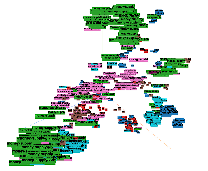
Step 4: exploring vector space with Projector
Now it’s time for a demonstration!
Using the vectorizer, we will generate embeddings for articles from the Reuters-21578 benchmark corpus.
To visualize and explore the embedding vector space in 3D, we will use a dimensionality reduction technique called T-SNE.
Let’s get the article embeddings first.
from nltk.corpus import reuters

nltk.download("reuters")
nltk.download("punkt")

max_samples = 256
categories = ['wheat', 'tea', 'strategic-metal',
              'housing', 'money-supply', 'fuel']

S, X, Y = [], [], []

for category in categories:
  print(category)

  sents = reuters.sents(categories=category)
  sents = [' '.join(sent) for sent in sents][:max_samples]
  X.append(bert_vectorizer(sents, verbose=True))
  Y += [category] * len(sents)
  S += sents

X = np.vstack(X)
X.shape
The interactive visualization of generated embeddings is available on the Embedding Projector.
From the link you can run T-SNE yourself or load a checkpoint using the bookmark in lower-right corner (loading works only on Chrome).
Building a supervised model with the generated features is straightforward:
from sklearn.linear_model import LogisticRegression
from sklearn.model_selection import train_test_split
from sklearn.metrics import classification_report

Xtr, Xts, Ytr, Yts = train_test_split(X, Y, random_state=34)

mlp = LogisticRegression()
mlp.fit(Xtr, Ytr)

print(classification_report(Yts, mlp.predict(Xts)))

'''
                 precision    recall  f1-score   support

           fuel       0.75      0.81      0.78        26
        housing       0.75      0.75      0.75        32
   money-supply       0.84      0.88      0.86        75
strategic-metal       0.86      0.90      0.88        48
            tea       0.90      0.82      0.86        44
          wheat       0.95      0.88      0.91        59

       accuracy                           0.85       284
      macro avg       0.84      0.84      0.84       284
   weighted avg       0.86      0.85      0.85       284

 '''
Step 5: building a search engine
Now, let’s say we have a knowledge base of 50k text samples and we need to answer queries based on this data, fast. How do we retrieve the sample most similar to a query from a text database? The answer is nearest neighbour search.
Formally, the search problem we will be solving is defined as follows:
given a set of points S in vector space M, and a query point Q ∈ M, find the closest point in S to Q. There are multiple ways to define ‘closest’ in vector space, we will use Euclidean distance.
So, to build an Search Engine for text we will follow these steps:
- Vectorize all samples from the knowledge base — that gives S
- Vectorize the query — that gives Q
- Compute euclidean distances D between Q and S
- Sort D in ascending order — providing indices of the most similar samples
- Retrieve labels for said samples from the knowledge base
To make the simple matter of implementing this a bit more exciting, we will do it in pure TensorFlow.
First, we create the placeholders for Q and S
dim = 1024
graph = tf.Graph()
sess = tf.InteractiveSession(graph=graph)

Q = tf.placeholder("float", [dim])
S = tf.placeholder("float", [None, dim])
Define euclidean distance computation
squared_distance = tf.reduce_sum(tf.pow(Q - S, 2), reduction_indices=1)
distance = tf.sqrt(squared_distance)
Finally, get the most similar sample indices
top_k = 3

top_neg_dists, top_indices = tf.math.top_k(tf.negative(distance), k=top_k)
top_dists = tf.negative(top_neg_dists)
Now that we have a basic retrieval algorithm set up, the question is:
can we make it run faster? With a tiny bit of math, we can.
Step 6: accelerating search with math
For a pair of vectors p and q, the euclidean distance is defined as follows:
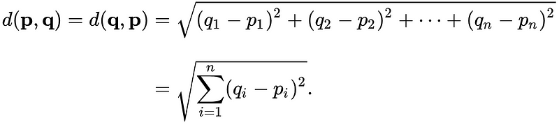
Which is exactly how we did compute it in Step 4.
However, since p and q are vectors, we can expand and rewrite this:

where ⟨…⟩ denotes inner product.
In TensorFlow this can be written as follows:
Q = tf.placeholder("float", [dim])
S = tf.placeholder("float", [None, dim])

Qr = tf.reshape(Q, (1, -1))

PP = tf.keras.backend.batch_dot(S, S, axes=1)
QQ = tf.matmul(Qr, tf.transpose(Qr))
PQ = tf.matmul(S, tf.transpose(Qr))

distance = PP - 2 * PQ + QQ
distance = tf.sqrt(tf.reshape(distance, (-1,)))

top_neg_dists, top_indices = tf.math.top_k(tf.negative(distance), k=top_k)
By the way, in the formula above PP and QQ are actually squared L2 norms of the respective vectors. If both vectors are L2 normalized, then PP = QQ = 1. That gives an interesting relation between inner product and euclidean distance:

However, doing L2 normalization discards the information about vector magnitude which in many cases is undesirable .
Instead, we may notice that as long as the knowledge base does not change, PP, its squared vector norm, also remains constant. So, instead of recomputing it every time we can just do it once and then use the precomputed result further accelerating the distance computation.
Now let us put it all together.
class L2Retriever:
    def __init__(self, dim, top_k=3, use_norm=False, use_gpu=True):
        self.dim = dim
        self.top_k = top_k
        self.use_norm = use_norm
        config = tf.ConfigProto(
            device_count={'GPU': (1 if use_gpu else 0)}
        )
        config.gpu_options.allow_growth = True
        self.session = tf.Session(config=config)

        self.norm = None
        self.query = tf.placeholder("float", [self.dim])
        self.kbase = tf.placeholder("float", [None, self.dim])

        self.build_graph()

    def build_graph(self):

        if self.use_norm:
            self.norm = tf.placeholder("float", [None, 1])

        distance = dot_l2_distances(self.kbase, self.query, self.norm)
        top_neg_dists, top_indices = tf.math.top_k(tf.negative(distance), k=self.top_k)
        top_dists = tf.negative(top_neg_dists)

        self.top_distances = top_dists
        self.top_indices = top_indices

    def predict(self, kbase, query, norm=None):
        query = np.squeeze(query)
        feed_dict = {self.query: query, self.kbase: kbase}
        if self.use_norm:
          feed_dict[self.norm] = norm

        I, D = self.session.run([self.top_indices, self.top_distances],
                                feed_dict=feed_dict)

        return I, D

def dot_l2_distances(kbase, query, norm=None):
    query = tf.reshape(query, (1, -1))

    if norm is None:
      XX = tf.keras.backend.batch_dot(kbase, kbase, axes=1)
    else:
      XX = norm
    YY = tf.matmul(query, tf.transpose(query))
    XY = tf.matmul(kbase, tf.transpose(query))

    distance = XX - 2 * XY + YY
    distance = tf.sqrt(tf.reshape(distance, (-1,)))

    return distance
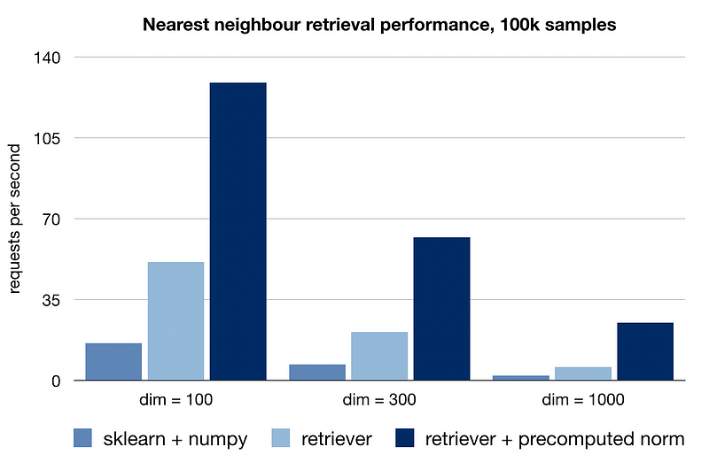
Naturally, you could use this implementation with any vectorizer model, not just BERT. It is quite effective at nearest neighbour retrieval, being able to process dozens of requests per second on a 2-core Colab CPU.
Example: movie recommendation system
For this example we will use a dataset of movie summaries from IMDB. Using the NLU and Retriever modules, we will build a movie recommendation system that suggests movies with similar plot features.
First, let’s download and prepare the IMDB dataset.
import pandas as pd
import json

!wget http://www.cs.cmu.edu/~ark/personas/data/MovieSummaries.tar.gz
!tar -xvzf MovieSummaries.tar.gz

plots_df = pd.read_csv('MovieSummaries/plot_summaries.txt', sep='\t', header=None)
meta_df = pd.read_csv('MovieSummaries/movie.metadata.tsv', sep='\t', header=None)

plot = {}
metadata = {}
movie_data = {}

for movie_id, movie_plot in plots_df.values:
  plot[movie_id] = movie_plot

for movie_id, movie_name, movie_genre in meta_df[[0,2,8]].values:
  genre = list(json.loads(movie_genre).values())
  if len(genre):
    metadata[movie_id] = {"name": movie_name,
                          "genre": genre}

for movie_id in set(plot.keys())&set(metadata.keys()):
  movie_data[metadata[movie_id]['name']] = {"genre": metadata[movie_id]['genre'],
                                            "plot": plot[movie_id]}

X, Y, names = [], [], []

for movie_name, movie_meta in movie_data.items():
  X.append(movie_meta['plot'])
  Y.append(movie_meta['genre'])
  names.append(movie_name)
Vectorize movie plots with the BERT NLU module:
X_vect = bert_vectorizer(X, verbose=True)
Finally, using the L2Retriever, find movies with plot vectors most similar to the query movie, and return it to user.
def buildMovieRecommender(movie_names, vectorized_plots, top_k=10):
  retriever = L2Retriever(vectorized_plots.shape[1], use_norm=True, top_k=top_k, use_gpu=False)
  vectorized_norm = np.sum(vectorized_plots**2, axis=1).reshape((-1,1))

  def recommend(query):
    try:
      idx = retriever.predict(vectorized_plots,
                              vectorized_plots[movie_names.index(query)],
                              vectorized_norm)[0][1:]
      for i in idx:
        print(names[i])
    except ValueError:
      print("{} not found in movie db. Suggestions:")
      for i, name in enumerate(movie_names):
        if query.lower() in name.lower():
          print(i, name)

  return recommend
Let’s check it out!
>>> recommend = buildMovieRecommender(names, X_vect)
>>> recommend("The Matrix")
Impostor
Immortel
Saturn 3
Terminator Salvation
The Terminator
Logan's Run
Genesis II
Tron: Legacy
Blade Runner
Models built with the features extracted from BERT perform adequately on classification and retrieval tasks. While their performance can be further improved by fine-tuning, the described approach to text feature extraction provides a solid unsupervised baseline for downstream NLP solutions.