ADBMS-1

techworldthink

Q1 : Define weak entity set with an example

An entity set may be of the following two types-

Strong entity set
Weak entity set

1. Strong Entity Set-

A strong entity set is an entity set that contains sufficient attributes to uniquely identify all its entities.
In other words, a primary key exists for a strong entity set.
Primary key of a strong entity set is represented by underlining it.

Symbols Used-

A single rectangle is used for representing a strong entity set.
A diamond symbol is used for representing the relationship that exists between two strong entity sets.
A single line is used for representing the connection of the strong entity set with the relationship set.
A double line is used for representing the total participation of an entity set with the relationship set.
Total participation may or may not exist in the relationship.

Example-

Consider the following ER diagram-

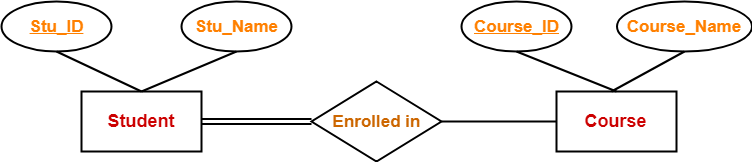
In this ER diagram,

Two strong entity sets “Student” and “Course” are related to each other.
Student ID and Student name are the attributes of entity set “Student”.
Student ID is the primary key using which any student can be identified uniquely.
Course ID and Course name are the attributes of entity set “Course”.
Course ID is the primary key using which any course can be identified uniquely.
Double line between Student and relationship set signifies total participation.
It suggests that each student must be enrolled in at least one course.
Single line between Course and relationship set signifies partial participation.
It suggests that there might exist some courses for which no enrollments are made.

2. Weak Entity Set-

A weak entity set is an entity set that does not contain sufficient attributes to uniquely identify its entities.
In other words, a primary key does not exist for a weak entity set.
However, it contains a partial key called as a discriminator.
Discriminator can identify a group of entities from the entity set.
Discriminator is represented by underlining with a dashed line.

NOTE-

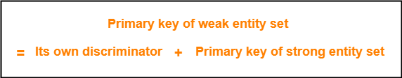
The combination of discriminator and primary key of the strong entity set makes it possible to uniquely identify all entities of the weak entity set.
Thus, this combination serves as a primary key for the weak entity set.
Clearly, this primary key is not formed by the weak entity set completely.

Symbols Used-

A double rectangle is used for representing a weak entity set.
A double diamond symbol is used for representing the relationship that exists between the strong and weak entity sets and this relationship is known as identifying relationship.
A double line is used for representing the connection of the weak entity set with the relationship set.
Total participation always exists in the identifying relationship.

Example-

Consider the following ER diagram-

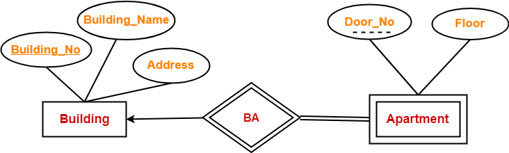
In this ER diagram,

One strong entity set “Building” and one weak entity set “Apartment” are related to each other.
Strong entity set “Building” has building number as its primary key.
Door number is the discriminator of the weak entity set “Apartment”.
This is because door number alone can not identify an apartment uniquely as there may be several other buildings having the same door number.
Double line between Apartment and relationship set signifies total participation.
It suggests that each apartment must be present in at least one building.
Single line between Building and relationship set signifies partial participation.
It suggests that there might exist some buildings which has no apartment.

Q2 : Levels of Data abstraction

Database systems comprise complex data-structures. In order to make the system efficient in terms of retrieval of data, and reduce complexity in terms of usability of users, developers use abstraction i.e. hide irrelevant details from the users. This approach simplifies database design.

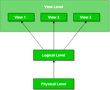
There are mainly 3 levels of data abstraction:

Physical: This is the lowest level of data abstraction. It tells us how the data is actually stored in memory. The access methods like sequential or random access and file organization methods like B+ trees, hashing used for the same. Usability, size of memory, and the number of times the records are factors that we need to know while designing the database.

Suppose we need to store the details of an employee. Blocks of storage and the amount of memory used for these purposes are kept hidden from the user.

Logical: This level comprises the information that is actually stored in the database in the form of tables. It also stores the relationship among the data entities in relatively simple structures. At this level, the information available to the user at the view level is unknown.

We can store the various attributes of an employee and relationships, e.g. with the manager can also be stored.

View: This is the highest level of abstraction. Only a part of the actual database is viewed by the users. This level exists to ease the accessibility of the database by an individual user. Users view data in the form of rows and columns. Tables and relations are used to store data. Multiple views of the same database may exist. Users can just view the data and interact with the database, storage and implementation details are hidden from them.

The main purpose of data abstraction is to achieve data independence in order to save time and cost required when the database is modified or altered.

We have namely two levels of data independence arising from these levels of abstraction :

Physical level data independence: It refers to the characteristic of being able to modify the physical schema without any alterations to the conceptual or logical schema, done for optimization purposes, e.g., Conceptual structure of the database would not be affected by any change in storage size of the database system server. Changing from sequential to random access files is one such example. These alterations or modifications to the physical structure may include:

Utilizing new storage devices.
Modifying data structures used for storage.
Altering indexes or using alternative file organization techniques etc.

Logical level data independence: It refers characteristic of being able to modify the logical schema without affecting the external schema or application program. The user view of the data would not be affected by any changes to the conceptual view of the data. These changes may include insertion or deletion of attributes, altering table structures entities or relationships to the logical schema, etc.

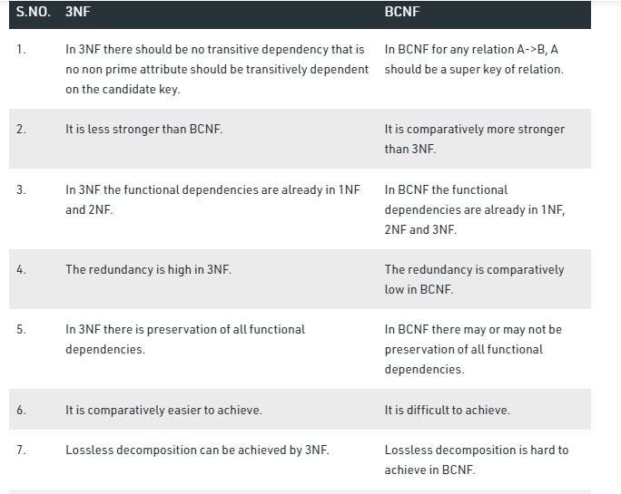
Q3 : BCNF vs 3NF

Q4 : Functional Dependency

The functional dependency is a relationship that exists between two attributes. It typically exists between the primary key and non-key attribute within a table.

X → Y

The left side of FD is known as a determinant, the right side of the production is known as a dependent.

For example:

Assume we have an employee table with attributes: Emp_Id, Emp_Name, Emp_Address.

Here Emp_Id attribute can uniquely identify the Emp_Name attribute of employee table because if we know the Emp_Id, we can tell that employee name associated with it.

Functional dependency can be written as:

Emp_Id → Emp_Name

Types of Functional dependency

1. Trivial functional dependency

2. Non-trivial functional dependency

1. Trivial functional dependency

A → B has trivial functional dependency if B is a subset of A.
The following dependencies are also trivial like: A → A, B → B

Example:

Consider a table with two columns Employee_Id and Employee_Name.

{Employee_id, Employee_Name} → Employee_Id is a trivial functional dependency as Employee_Id is a subset of {Employee_Id, Employee_Name}. Also, Employee_Id → Employee_Id and Employee_Name → Employee_Name are trivial dependencies too.

2. Non-trivial functional dependency

A → B has a non-trivial functional dependency if B is not a subset of A.
When A intersection B is NULL, then A → B is called as complete non-trivial.

Example:

ID → Name,
Name → DOB

Q5 : ACID properties of transactions

DBMS is the management of data that should remain integrated when any changes are done in it. It is because if the integrity of the data is affected, whole data will get disturbed and corrupted. Therefore, to maintain the integrity of the data, there are four properties described in the database management system, which are known as the ACID properties. The ACID properties are meant for the transaction that goes through a different group of tasks, and there we come to see the role of the ACID properties.

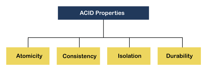
1) Atomicity: The term atomicity defines that the data remains atomic. It means if any operation is performed on the data, either it should be performed or executed completely or should not be executed at all. It further means that the operation should not break in between or execute partially. In the case of executing operations on the transaction, the operation should be completely executed and not partially.

2) Consistency: The word consistency means that the value should remain preserved always. In DBMS, the integrity of the data should be maintained, which means if a change in the database is made, it should remain preserved always. In the case of transactions, the integrity of the data is very essential so that the database remains consistent before and after the transaction. The data should always be correct.

3) Isolation: The term 'isolation' means separation. In DBMS, Isolation is the property of a database where no data should affect the other one and may occur concurrently. In short, the operation on one database should begin when the operation on the first database gets complete. It means if two operations are being performed on two different databases, they may not affect the value of one another. In the case of transactions, when two or more transactions occur simultaneously, the consistency should remain maintained. Any changes that occur in any particular transaction will not be seen by other transactions until the change is not committed in the memory.

4) Durability: Durability ensures the permanency of something. In DBMS, the term durability ensures that the data after the successful execution of the operation becomes permanent in the database. The durability of the data should be so perfect that even if the system fails or leads to a crash, the database still survives. However, if gets lost, it becomes the responsibility of the recovery manager for ensuring the durability of the database. For committing the values, the COMMIT command must be used every time we make changes.

Q6 : Deadlocks in DBMS , stratergies for managing deadlocks.

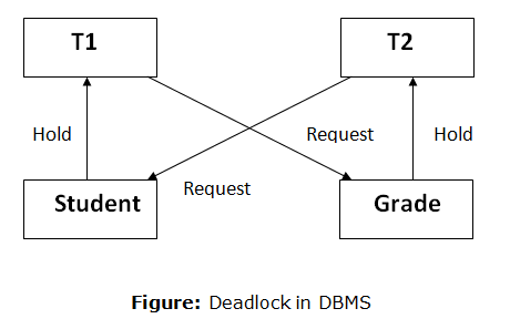
A deadlock is a condition where two or more transactions are waiting indefinitely for one another to give up locks. Deadlock is said to be one of the most feared complications in DBMS as no task ever gets finished and is in waiting state forever.

For example: In the student table, transaction T1 holds a lock on some rows and needs to update some rows in the grade table. Simultaneously, transaction T2 holds locks on some rows in the grade table and needs to update the rows in the Student table held by Transaction T1.

Now, the main problem arises. Now Transaction T1 is waiting for T2 to release its lock and similarly, transaction T2 is waiting for T1 to release its lock. All activities come to a halt state and remain at a standstill. It will remain in a standstill until the DBMS detects the deadlock and aborts one of the transactions.

Deadlock Avoidance

When a database is stuck in a deadlock state, then it is better to avoid the database rather than aborting or restating the database. This is a waste of time and resource.
Deadlock avoidance mechanism is used to detect any deadlock situation in advance. A method like "wait for graph" is used for detecting the deadlock situation but this method is suitable only for the smaller database. For the larger database, deadlock prevention method can be used.

Deadlock Detection

In a database, when a transaction waits indefinitely to obtain a lock, then the DBMS should detect whether the transaction is involved in a deadlock or not. The lock manager maintains a Wait for the graph to detect the deadlock cycle in the database.

Wait for Graph

This is the suitable method for deadlock detection. In this method, a graph is created based on the transaction and their lock. If the created graph has a cycle or closed loop, then there is a deadlock.
The wait for the graph is maintained by the system for every transaction which is waiting for some data held by the others. The system keeps checking the graph if there is any cycle in the graph.

The wait for a graph for the above scenario is shown below:

Deadlock Prevention

Deadlock prevention method is suitable for a large database. If the resources are allocated in such a way that deadlock never occurs, then the deadlock can be prevented.
The Database management system analyzes the operations of the transaction whether they can create a deadlock situation or not. If they do, then the DBMS never allowed that transaction to be executed.

Wait-Die scheme

In this scheme, if a transaction requests for a resource which is already held with a conflicting lock by another transaction then the DBMS simply checks the timestamp of both transactions. It allows the older transaction to wait until the resource is available for execution.

Let's assume there are two transactions Ti and Tj and let TS(T) is a timestamp of any transaction T. If T2 holds a lock by some other transaction and T1 is requesting for resources held by T2 then the following actions are performed by DBMS:

Check if TS(Ti) < TS(Tj) - If Ti is the older transaction and Tj has held some resource, then Ti is allowed to wait until the data-item is available for execution. That means if the older transaction is waiting for a resource which is locked by the younger transaction, then the older transaction is allowed to wait for resource until it is available.
Check if TS(Ti) < TS(Tj) - If Ti is older transaction and has held some resource and if Tj is waiting for it, then Tj is killed and restarted later with the random delay but with the same timestamp.

Wound wait scheme

In wound wait scheme, if the older transaction requests for a resource which is held by the younger transaction, then older transaction forces younger one to kill the transaction and release the resource. After the minute delay, the younger transaction is restarted but with the same timestamp.
If the older transaction has held a resource which is requested by the Younger transaction, then the younger transaction is asked to wait until older releases it.

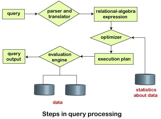
Q7 : Diagrammatically represent the basic steps in query processing.

Query Processing is the activity performed in extracting data from the database. In query processing, it takes various steps for fetching the data from the database. The steps involved are:

Parsing and translation
Optimization
Evaluation

The query processing works in the following way:

Parsing and Translation

As query processing includes certain activities for data retrieval. Initially, the given user queries get translated in high-level database languages such as SQL. It gets translated into expressions that can be further used at the physical level of the file system. After this, the actual evaluation of the queries and a variety of query -optimizing transformations and takes place. Thus before processing a query, a computer system needs to translate the query into a human-readable and understandable language. Consequently, SQL or Structured Query Language is the best suitable choice for humans. But, it is not perfectly suitable for the internal representation of the query to the system. Relational algebra is well suited for the internal representation of a query. The translation process in query processing is similar to the parser of a query. When a user executes any query, for generating the internal form of the query, the parser in the system checks the syntax of the query, verifies the name of the relation in the database, the tuple, and finally the required attribute value. The parser creates a tree of the query, known as 'parse-tree.' Further, translate it into the form of relational algebra. With this, it evenly replaces all the use of the views when used in the query.

Thus, we can understand the working of a query processing in the below-described diagram:

Suppose a user executes a query. As we have learned that there are various methods of extracting the data from the database. In SQL, a user wants to fetch the records of the employees whose salary is greater than or equal to 10000. For doing this, the following query is undertaken:

select emp_name from Employee where salary>10000;

Thus, to make the system understand the user query, it needs to be translated in the form of relational algebra. We can bring this query in the relational algebra form as:

σsalary>10000 (πsalary (Employee))
πsalary (σsalary>10000 (Employee))

After translating the given query, we can execute each relational algebra operation by using different algorithms. So, in this way, a query processing begins its working.

Evaluation

For this, with addition to the relational algebra translation, it is required to annotate the translated relational algebra expression with the instructions used for specifying and evaluating each operation. Thus, after translating the user query, the system executes a query evaluation plan.

Query Evaluation Plan

In order to fully evaluate a query, the system needs to construct a query evaluation plan.
The annotations in the evaluation plan may refer to the algorithms to be used for the particular index or the specific operations.
Such relational algebra with annotations is referred to as Evaluation Primitives. The evaluation primitives carry the instructions needed for the evaluation of the operation.
Thus, a query evaluation plan defines a sequence of primitive operations used for evaluating a query. The query evaluation plan is also referred to as the query execution plan.
A query execution engine is responsible for generating the output of the given query. It takes the query execution plan, executes it, and finally makes the output for the user query.

Optimization

The cost of the query evaluation can vary for different types of queries. Although the system is responsible for constructing the evaluation plan, the user does need not to write their query efficiently.
Usually, a database system generates an efficient query evaluation plan, which minimizes its cost. This type of task performed by the database system and is known as Query Optimization.
For optimizing a query, the query optimizer should have an estimated cost analysis of each operation. It is because the overall operation cost depends on the memory allocations to several operations, execution costs, and so on.

Finally, after selecting an evaluation plan, the system evaluates the query and produces the output of the query.

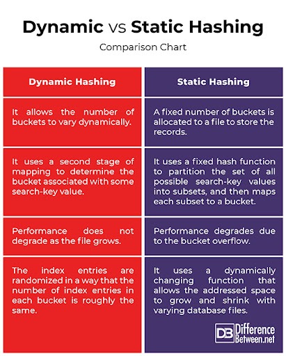
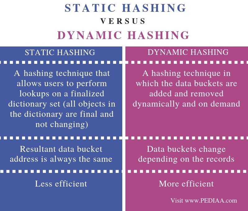
Q8 : Static vs Dynamic Hashing

In DBMS, hashing is a technique to directly search the location of desired data on the disk without using index structure. Hashing method is used to index and retrieve items in a database as it is faster to search that specific item using the shorter hashed key instead of using its original value. Data is stored in the form of data blocks whose address is generated by applying a hash function in the memory location where these records are stored known as a data block or data bucket.

Why do we need Hashing?

Here, are the situations in the DBMS where you need to apply the Hashing method:

For a huge database structure, it’s tough to search all the index values through all its level and then you need to reach the destination data block to get the desired data.
Hashing method is used to index and retrieve items in a database as it is faster to search that specific item using the shorter hashed key instead of using its original value.
Hashing is an ideal method to calculate the direct location of a data record on the disk without using index structure.
It is also a helpful technique for implementing dictionaries.

There are mainly two types of SQL hashing methods:

Static Hashing
Dynamic Hashing

Static Hashing

In the static hashing, the resultant data bucket address will always remain the same.

Therefore, if you generate an address for say Student_ID = 10 using hashing function mod(3), the resultant bucket address will always be 1. So, you will not see any change in the bucket address.

Therefore, in this static hashing method, the number of data buckets in memory always remains constant.

Static Hash Functions

Inserting a record: When a new record requires to be inserted into the table, you can generate an address for the new record using its hash key. When the address is generated, the record is automatically stored in that location.
Searching: When you need to retrieve the record, the same hash function should be helpful to retrieve the address of the bucket where data should be stored.
Delete a record: Using the hash function, you can first fetch the record which is you wants to delete. Then you can remove the records for that address in memory.

Static hashing is further divided into

Open hashing
Close hashing.

Open Hashing

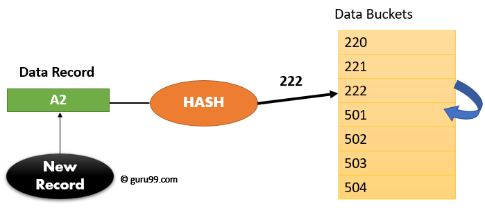
In Open hashing method, Instead of overwriting older one the next available data block is used to enter the new record, This method is also known as linear probing.

For example, A2 is a new record which you wants to insert. The hash function generates address as 222. But it is already occupied by some other value. That’s why the system looks for the next data bucket 501 and assigns A2 to it.

Close Hashing

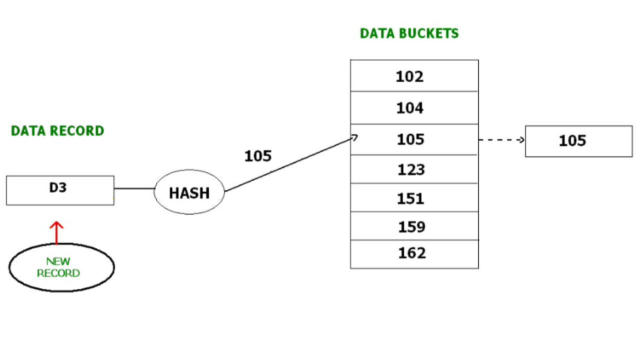
In Closed hashing method, a new data bucket is allocated with same address and is linked it after the full data bucket. This method is also known as overflow chaining.

For example, we have to insert a new record D3 into the tables. The static hash function generates the data bucket address as 105. But this bucket is full to store the new data. In this case is a new data bucket is added at the end of 105 data bucket and is linked to it. Then new record D3 is inserted into the new bucket.

Quadratic probing :

Quadratic probing is very much similar to open hashing or linear probing. Here, The only difference between old and new bucket is linear. Quadratic function is used to determine the new bucket address.

Double Hashing :

Double Hashing is another method similar to linear probing. Here the difference is fixed as in linear probing, but this fixed difference is calculated by using another hash function. That’s why the name is double hashing.

2 Dynamic Hashing

The drawback of static hashing is that that it does not expand or shrink dynamically as the size of the database grows or shrinks. In Dynamic hashing, data buckets grows or shrinks (added or removed dynamically) as the records increases or decreases. Dynamic hashing is also known as extended hashing.

Dynamic hashing offers a mechanism in which data buckets are added and removed dynamically and on demand. In this hashing, the hash function helps you to create a large number of values.

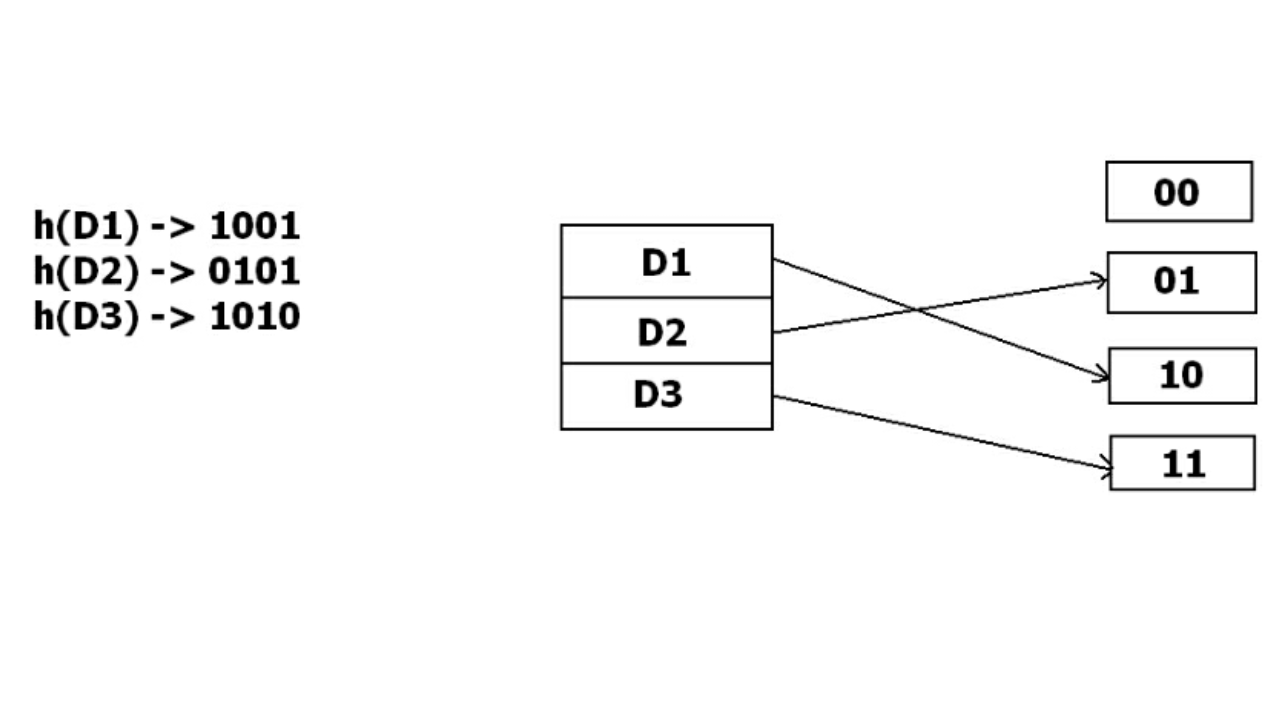
In dynamic hashing, the hash function is made to produce a large number of values. For Example, there are three data records D1, D2 and D3 . The hash function generates three addresses 1001, 0101 and 1010 respectively. This method of storing considers only part of this address – especially only first one bit to store the data. So it tries to load three of them at address 0 and 1.

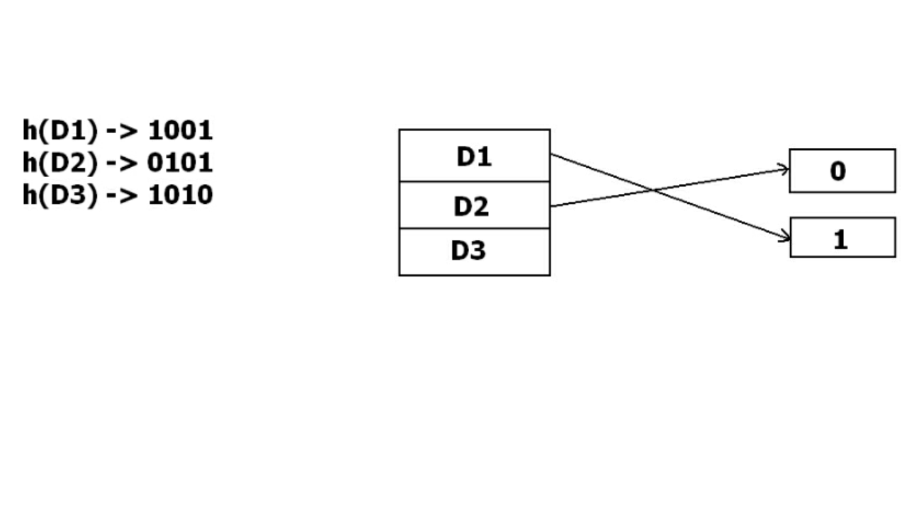
But the problem is that No bucket address is remaining for D3. The bucket has to grow dynamically to accommodate D3. So it changes the address have 2 bits rather than 1 bit, and then it updates the existing data to have 2 bit address. Then it tries to accommodate D3.

Q9 : Different types of Distributed Databases

A distributed database is basically a database that is not limited to one system, it is spread over different sites, i.e, on multiple computers or over a network of computers. A distributed database system is located on various sites that don’t share physical components. This may be required when a particular database needs to be accessed by various users globally. It needs to be managed such that for the users it looks like one single database.

1. Homogeneous Database:

In a homogeneous database, all different sites store database identically. The operating system, database management system and the data structures used – all are same at all sites. Hence, they’re easy to manage.

2. Heterogeneous Database:

In a heterogeneous distributed database, different sites can use different schema and software that can lead to problems in query processing and transactions. Also, a particular site might be completely unaware of the other sites. Different computers may use a different operating system, different database application. They may even use different data models for the database. Hence, translations are required for different sites to communicate.

Distributed Data Storage :

There are 2 ways in which data can be stored on different sites. These are:

1. Replication –

In this approach, the entire relation is stored redundantly at 2 or more sites. If the entire database is available at all sites, it is a fully redundant database. Hence, in replication, systems maintain copies of data.

This is advantageous as it increases the availability of data at different sites. Also, now query requests can be processed in parallel.

However, it has certain disadvantages as well. Data needs to be constantly updated. Any change made at one site needs to be recorded at every site that relation is stored or else it may lead to inconsistency. This is a lot of overhead. Also, concurrency control becomes way more complex as concurrent access now needs to be checked over a number of sites.

2. Fragmentation –

In this approach, the relations are fragmented (i.e., they’re divided into smaller parts) and each of the fragments is stored in different sites where they’re required. It must be made sure that the fragments are such that they can be used to reconstruct the original relation (i.e, there isn’t any loss of data).

Fragmentation is advantageous as it doesn’t create copies of data, consistency is not a problem.

Fragmentation of relations can be done in two ways:

Horizontal fragmentation – Splitting by rows –
The relation is fragmented into groups of tuples so that each tuple is assigned to at least one fragment.
Vertical fragmentation – Splitting by columns –
The schema of the relation is divided into smaller schemas. Each fragment must contain a common candidate key so as to ensure lossless join.

In certain cases, an approach that is hybrid of fragmentation and replication is used.

Q10 : Define Collection and Document in MongoDB

MongoDB stores documents in collections. Collections are analogous to tables in relational databases. If a collection does not exist, MongoDB creates the collection when you first store data for that collection.

db.myNewCollection2.insertOne( { x: 1 } )

Collection is a group of MongoDB documents. It is the equivalent of an RDBMS table. A collection exists within a single database. Collections do not enforce a schema. Documents within a collection can have different fields. Typically, all documents in a collection are of similar or related purpose.

A document is a set of key-value pairs. Documents have dynamic schema. Dynamic schema means that documents in the same collection do not need to have the same set of fields or structure, and common fields in a collection's documents may hold different types of data.

{
   _id: ObjectId(7df78ad8902c)
   title: 'MongoDB Overview', 
}