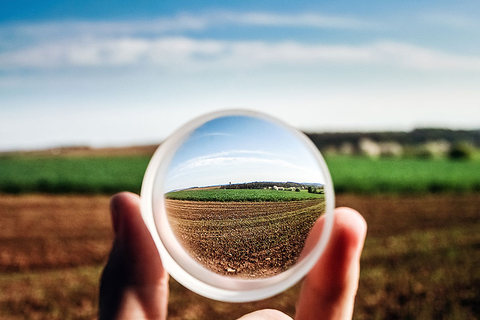
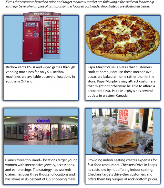
A Focused Coed Image

🛑 👉🏻👉🏻👉🏻 INFORMATION AVAILABLE CLICK HERE👈🏻👈🏻👈🏻

Search 123RF with an image instead of text. Try dragging an image to the search box.
264.687 matches including pictures of glimmer, twinkle, brilliance and physique
Need help? Contact your dedicated Account Manager
All rights reserved. © Inmagine Lab Pte Ltd 2021.

The synthetic aperture achieves fine cross-range resolution by adjusting the relative phase among signals received from various pulses and coherently summing them to achieve a focused image. A major source of uncertainty in the relative phase among these signals is the exact location of the radar antenna at the time of transmission and reception of each pulse. Location accuracy on the order of a fraction of a wavelength is necessary, perhaps to a few millimeters in the case of X-band operation at 10-GHz center frequency. Without this location accuracy, phase errors will exist across the azimuth signal aperture and cause image distortion, defocus, and loss of contrast. Other hardware and software sources of phase error also are likely to be present even in a well-designed system.
The high probability of significant phase error in the azimuth channel of a SAR system operating at fine resolution (typically better than 1-m azimuth resolution) necessitates the use of algorithms during or following image formation to measure and remove this phase error. We refer to the process that automatically estimates and compensates for phase error as autofocus. We describe two common autofocus algorithms in this chapter, the mapdrift algorithm and phase gradient autofocus (PGA). The mapdrift algorithm is ideal for detecting and removing low-frequency phase error that causes image defocus. By low frequency, we mean phase error that varies slowly (for example, a quadratic or cubic variation) over the aperture. PGA is an elegant algorithm designed to detect both low-frequency phase error and high-frequency phase error that varies rapidly over the aperture. High-frequency phase error primarily degrades image contrast.
Originating at Hughes Aircraft Corporation in the mid 1970s, the mapdrift algorithm became the first robust autofocus procedure to see widespread use in operational SAR systems. While mapdrift estimates quadratic and cubic phase errors best, it also extends to higher frequency phase error [9]. With the aid of Fig. 16, we illustrate use of the mapdrift concept to detect and estimate an azimuth quadratic phase error with center-to-edge phase of Q over an aperture of duration Ta. This error has the form exp (j2πkqx2) where x is the azimuth coordinate and kq is the quadratic phase coefficient being measured. In its quadratic mode, mapdrift begins by dividing the signal data into two halves (or subapertures) in azimuth, each of length Ta/2. Mapdrift forms separate, but similar, images (or maps) from each subaperture. This process degrades the azimuth resolution of each map by a factor of two relative to the full-aperture image. Viewed separately over each subaperture, the original phase effect includes identical constant and quadratic components but a linear component of opposite slope in each subaperture. Mapdrift exploits the fact that each subaperture possesses a different linear phase component. A measurement of the difference between the linear phase components over the two subapertures leads to an estimate of the original quadratic phase error over the full aperture. The constant phase component over each subaperture is inconsequential, while the quadratic phase component causes some defocus in the subaperture images that is not too troublesome.
FIGURE 16. Subaperture phase characteristics in mapdrift concept.
By the Fourier shift theorem, a linear phase in the signal domain causes a proportional shift in the image domain. By estimating the shift (or drift) between the two similar maps, the mapdrift algorithm estimates the difference in the linear phase component between the two subapertures. This difference is directly proportional to Q. Most implementations of mapdrift measure the drift between maps by locating the peak of the cross-correlation of the intensity (magnitude squared) maps. After mapdrift estimates the error, a subsequent step removes the error from the full data aperture by multiplying the original signal by a complex exponential of unity magnitude and phase equal to the negative of the estimated error. Typical implementations improve algorithm performance by iterating the process after removing the current error estimate. Use of more than two subapertures to extend the algorithm to higher frequency phase error is rare because of the availability of more capable higher order techniques, such as the PGA algorithm.
The PGA entered the SAR arena in 1989 as a method to estimate higher order phase errors in complex SAR signal data [10, 11]. Unlike mapdrift, PGA is a nonparametric technique in that it does not assume any particular functional model (for example, quadratic) for the phase error. PGA follows an iterative procedure to estimate the derivative (or phase gradient) of a phase error in one dimension. The underlying idea is simple. The phase of the signal that results from isolating a dominant scatterer within an image and inverse Fourier transforming it in azimuth is a measure of the azimuth phase error in the signal data.
The PGA iteration cycle begins with a complex image that is focused in range but possibly blurred in azimuth by the phase error being estimated. The basic procedure isolates (by windowing) the image samples containing the azimuth impulse response of the dominant scatterer within each range bin and inverse Fourier transforms the windowed samples. The PGA implementation estimates the phase error in azimuth by measuring the change (or gradient) in phase between adjacent samples of the inverse transformed signal in each range bin, averaging these measurements over all range bins, and integrating the average. The algorithm then removes the estimated phase error from the original SAR data and proceeds with the next iteration. A number of techniques are available for selecting the initial window width. Typical implementations of PGA decrease the window width following each iteration of the algorithm.
Figure 17 demonstrates use of PGA to focus a 0.3-m resolution stripmap image of the University of Michigan engineering campus. The image in Fig. 17A contains a higher order phase error in azimuth that seriously degrades image quality. Figure 17B shows the focused image that results after three iterations of the PGA algorithm. This comparison illustrates the ability of PGA to estimate higher order phase errors accurately. While the presence of numerous dominant scatterers in this example eases the focusing task considerably, PGA also exhibits robust performance against scenes without dominant scatterers.
FIGURE 17. Phase gradient autofocus algorithm example: (A) Input image degraded with simulated phase errors; (B) output image after autofocus.
URL: https://www.sciencedirect.com/science/article/pii/B9780121197926501273
Yoav Y. Schechner, Shree K. Nayar, in Image Fusion, 2008
Focusing is required in most cameras. Let the camera view an object at a distance sobject from the first (front) principal plane of the lens. A focused image of this object is formed at a distance simage behind the second (back) principal plane of the lens, as illustrated in Figure 8.3. For simplicity, consider first an aberration-free flat-field camera, having an effective focal length f. Then,
Figure 8.3. Geometry of a simple camera system.
Hence, simage is equivalent to sobject. The image is sensed by a detector array (e.g., a CCD), situated at a distance sdetector from the back principal plane. If sdetector = simage, then the detector array senses the focused image. Generally, however, sdetector ≠ simage. If |simage − sdetector| is sufficiently large, then the detector senses an image which is defocus blurred.
For a given sdetector, there is a small range of simage values for which the defocus blur is insignificant. This range is the depth of focus. Due to the equivalence of simage to sobject, this corresponds to a range of object distances which are imaged sharply on the detector array. This range is the depth of field (DOF). Hence, a single frame can generally capture in focus objects that are in this limited span. However, typically, different objects or points in the FOV have different distances sobject, extending beyond the DOF. Hence, while some objects in a frame are in focus, others are defocus blurred.
There is a common method to capture each object point in focus, using a stationary camera. In this method, the FOV is fixed, while K frames of the scene are acquired. In each frame, indexed k ε [1, K], the focus settings of the system change relative to the previous frame. Change of the settings can be achieved by varying sdetector, or f, or sobject, or any combination of them. This way, for any specific object point (x, y), there is a frame k(x, y) for which Equation (8.1) is approximated as
Figure 8.4. An image frame has a limited FOV of the scene (marked by
x∼
) and a limited DOF. By fusing differently focused images, the DOF can be extended by image post processing, but the FOV remains limited.
URL: https://www.sciencedirect.com/science/article/pii/B9780123725295000160
Another set of psychovisual experiments has determined what has come to be regarded as the spatial frequency response of the HVS. In these experiments, a uniform plane wave is presented to viewers at a given distance, and the angular period of the image focused on their retina is calculated. The question is at what intensity does the plane wave (sometimes called an optical grating) first become visible. The researcher then plots this value as a function of angular spatial frequency, expressed in units of cycles/degree. These values are then averaged over many observers to come up with a set of threshold values for the so-called standard observer. The reciprocal of this function is then taken as the human visual frequency response and called the contrast sensitivity function (CSF), as seen plotted in Figure 6.2–4, reprinted from [3, 4]. Of course, there must be a uniform background used that is of a prescribed value, on account of Weber's law. Otherwise the threshold would change. Also, for very low spatial frequencies, the threshold value should be given by Weber's observation, since he used a plain or flat background. The CSF is based on the assumption that the above-threshold sensitivity of the HVS is the same as the threshold sensitivity. In fact, this may not be the case, but it is the current working assumption. Another objection could be that the threshold may not be the same with two stimuli present (i.e., the sum of two different plane waves). Nevertheless, with the so-called linear hypothesis, we can weight a given disturbance presented to the HVS with a function that is the reciprocal of these threshold values and effectively normalize them. If the overall intensity is then gradually reduced, all the gratings will become invisible (not noticeable to about 50% of human observers with normal acuity) at the same point. In that sense then, the CSF is the frequency response of the HVS.
Figure 6.2–4. Contrast sensitivity measurements of van Ness and Bouman. (JOSA, 1967 [4])
with A = 2.6, α = 0.0192, f0 = 8.772, and β = 1.1. (Here, f = ω/2π.) In this formula, the peak occurs at fr = 8(cycles/degree) and the function is normalized to maximum value 1. A linear amplitude plot of this function is given in Figure 6.2–5. Note that sensitivity is quite low at zero spatial frequency, so some kind of spatial structure or texture is almost essential if a feature is to be noticed by our HVS.
Figure 6.2–5. Plot of the Mannos and Sakrison CSF [5].
URL: https://www.sciencedirect.com/science/article/pii/B9780123814203000060
In the synchronous-beam-movement-type (SBM-type) AWGs [26, 27], input position of the beam moves synchronously with the wavelength change of the signal. Then, output beam lies in a fixed position independent of wavelength within one channel span. Figure 9.58 shows the schematic configuration of the first kind of SBM-type AWG [26]. Two AWGs are arranged in tandem, and the image of the first AWG forms the source for the second AWG. The image of the first AWG is created on the dotted line AA′. Free spectral range (FSR) of AWG1 is designed to be equal to the channel spacing of AWG2. Focused images for 100-GHz-spacing SBM-type AWG are calculated by the BPM simulations. The first AWG is a 1-ch, 100-GHz and the second AWG is a 64-ch, 100-GHz AWG. Figure 9.59 shows focused images (optical intensity) on AA′ and BB′ for three spectral components δλ = −0.2 nm, 0.0 nm and +0.2 nm, respectively. Three peaks in Fig. 9.59 are images for three diffraction orders. When wavelength λ decreases (increases) within a channel, focused image of AWG1 moves upward (downward) on the dotted line AA′ as shown in Fig. 9.59(a). When change of wavelength δλ is ignored, the second image on the line BB′ moves in the opposite direction to that on AA′ as shown in Fig. 9.59(b) according to Eq. (9.4). However, when wavelength change δλ. is taken into account, the focused spot on BB′ moves upward (downward) according to Eq. (9.5) and the main spot stays at the center of the output waveguide as shown in Fig. 9.59(c). Then, beam movement in the first AWG precisely cancels the focused spot movement on BB′ and enables us to obtain flat spectral response AWG without causing an extra loss increase.
Figure 9.58. Schematic configuration of the first kind of SBM-type AWG.
Figure 9.59. Focused images on the dotted lines A–A′ and B–B′ for three spectral components δλ = −0.2 nm, 0.0 nm and + 0.2 nm, respectively.
It is clear that the neighboring two peaks cause substantial crosstalk degradation. Therefore, a filter having proper width should be incorporated in the focal plane AA′ to eliminate the neighboring two images. Hatched regions in Fig. 9.60 show the filters to improve the crosstalk characteristics. Figure 9.60 shows focused images on AA′ and BB′ when filters are placed for three spectral components δλ = −0.2nm, 0.0nm and + 0.2nm, respectively. Overlap integral of the focused field (Fig. 9.60(c)) with the LNM in the output-tapered waveguide gives the spectral response as shown in Fig. 9.61. Theoretical loss of the current model of AWG is about 4.0 dB, which includes (a) imperfect light capture loss at the first slab of AWG, (about 0.85 dB), (b) blocking loss of the neighboring diffraction orders at the second slab of AWG, (about 1.45 dB), (c) imperfect light capture loss at the first slab of AWG2 (about 0.85 dB), and (d) sidelobe loss as shown in Fig. 9.19 (about 0.85 dB), respectively.
Figure 9.60. Focused images on A–A′ and B–B′ when filters are placed for three spectral components δλ = −0.2 nm, 0.0 nm and + 0.2 nm, respectively.
Figure 9.61. Theoretical flat spectral response of the first kind of SBM-type AWG with 100-GHz channel spacing.
Figure 9.62 shows the schematic configuration of the second kind of SBM-type AWG [27]. Asymmetrical Mach–Zehnder (AMZ) interferometer and AWG are arranged in tandem, and the image of AMZ forms the source for the AWG. The image of AMZ is created on the dotted line AA′. FSR of AMZ is designed to be equal to the channel spacing of the AWG. Path length difference in AMZ is about 2.07 mm so as to realize FSR= 100GHz. Operational principle of the present SBM-type AWG is similar to that of the previous case. Focused images for 100-GHz-spacing SBM-type 64-ch, 100-GHz AWG are calculated by the BPM simulations. Figure 9.63 shows field intensity on AA′ and BB′ for three spectral components Sλ = −0.2nm, 0.0nm and + 0.2nm, respectively. Here, waveguide gap and 3-dB coupler length of AMZ are 1.5 μm and 360 μm for the channel waveguide having 2a = 7.0 μm, 2t = 6.0 μm and Δ = 0.75%, respectively. Figure 9.63(b) shows the image on BB′ when wavelength change δλ is ignored. When wavelength change δλ is taken into account, the image stays at the center of the output waveguide as shown in Fig. 9.63(c). Field distribution at δλ = 0.0nm is essentially double peaked, since light is localized to each core of the 3-dB coupler. Then, aperture width of the output-tapered waveguide is optimized to 14.5 μm in order to capture the double-peaked light properly. Overlap integral of the focused field (Fig. 9.63(c)) with the LNM in the output-tapered waveguide gives the spectral response as shown in Fig. 9.64. Theoretical loss of the current model of AWG is about 2.5 dB, which includes (a) imperfect light capture loss at the first slab (about 0.85 dB), and (b) field mismatch loss between the optical field and the local normal mode (about 0.8 dB), and (c) sidelobe loss as shown in Fig. 9.19 (about 0.85 dB). Crosstalk degradation at around −35 dB level could be eliminated by incorporating a light blocking filter on the A A′ plane.
Figure 9.62. Schematic configuration of the second kind of SBM-type AWG.
Figure 9.63. Focused images on the dotted lines A–A′ and B–B′ for three spectral components δλ = −0.2nm, O.Onm and + 0.2nm, respectively.
Figure 9.64. Theoretical flat spectral response of the second kind of SBM-type AWG with 100-GHz channel spacing.
URL: https://www.sciencedirect.com/science/article/pii/B9780125250962500106
As previously discussed in Section 1.3.1, the use of extreme zoom levels significantly reduces the depth of field. To correctly adjust the focus distance to the subject position in the scene, two different strategies can be exploited: (i) auto-focus and (ii) manual focus.
In the former, the focus adjustment is guided by an image contrast maximization search. Despite being highly effective in wide-view cameras, this approach fails to provide focused images of moving subjects when using extreme zoom magnifications. Firstly, the reduced field of view of the camera significantly reduces the amount of time the subject is imaged (approximately 1 s), and the auto-focus mechanism is not fast enough (approximately 2 s) to seamlessly frame the subject over time. Secondly, motion also introduces blur in the image which may mislead the contrast adjustment scheme.
As an alternative, the focus lens can be manually adjusted with respect to the distance of the subject to the camera. Given the 3D position of the subject, it is possible to infer its distance to the camera. Then, focus is dynamically adjusted using a function relating the subject's distance and the focus lens position. In this strategy, the estimation of a 3D subject position is regarded as the major bottleneck since it depends on the use of stereo reconstruction techniques. However, this issue has been progressively addressed by the state-of-the-art methods since 3D information is critical for accurate PTZ-based systems.
URL: https://www.sciencedirect.com/science/article/pii/B9780081007051000014
Bijoy Bhattacharyya, Biswanath
Porno Movies Incest
3d Incest Porn Video
Porno Brazil's
Big Clit Pictures
Cartoon Sex Teen Titans
Focused Stock Photos. Royalty Free Focused Images
Focused Image - an overview | ScienceDirect Topics
focused image - Spanish translation – Linguee
30,000+ Best Focus Photos · Free to Download · Pexels ...
1000+ Free Focused Stock Photos | Icons8
Customer Focused Photos and Premium High ... - Getty Images
Image focus | OptoWiki Knowledge Base
200+ Free Focused & Cat Images - Pixabay
All-in-Focus Imaging Using a Series of Images on Different ...
LunaPic | Free Online Photo Editor | Adjust Focus
A Focused Coed Image