OT ..

UNIT 1

OPERATION RESEARCH: Operations research (OR) is an analytical method of problem-solving and decision-making that is useful in the management of organizations. In operations research, problems are broken down into basic components and then solved in defined steps by mathematical analysis.

Characteristics of Operations Research :

1) System (or Executive) Orientation of OR
2) The Use of Interdisciplinary Teams
3) Application of Scientific Method
4) Uncovering of New Problems
5) Improvement in the Quality of Decisions
6) Use of Computer
7) Quantitative Solutions
8) Human Factors

DECISION VARIABLES: Decision variables describe the quantities that the decision-makers would like to determine. They are the unknowns of a mathematical programming model. Typically we will determine their optimum values with an optimization method. In a general model, decision variables are given algebraic designations such as.

OBJECTIVE FUNCTION: The objective function evaluates some quantitative criterion of immediate importance such as cost, profit, utility, or yield. The general linear objective function can be written as Here is the coefficient of the jth decision variable. The criterion selected can be either maximized or minimized

CONSTRAINTS: A constraint is inequality or equality defining limitations on decisions. Constraints arise from a variety of sources such as limited resources, contractual obligations, or physical laws. In general, an LP is said to have m linear constraints that can be stated as One of the three relations shown in the large brackets that must be chosen for each constraint. The number is called a "technological coefficient," and the number is called the "right-side" value of the ith constraint. Strict inequalities (<, >, and ) are not permitted. When formulating a model, it is good practice to give a name to each constraint that reflects its purpose.

SIMPLE UPPER BOUND: Associated with each variable, maybe a specified quantity, , that limits its value from above; When a simple upper is not specified for a variable, the variable is said to be unbounded from above.

NONNEGATIVITY RESTRICTIONS: In most practical problems the variables are required to be nonnegative; This special kind of constraint is called a nonnegativity restriction. Sometimes variables are required to be nonpositive or, in fact, maybe unrestricted (allowing any real value).

COMPLETE LINEAR PROGRAMMING MODEL: Combining the mentioned components into a single statement gives: The constraints, including nonnegativity and simple upper bounds, define the feasible region of a problem.

PARAMETERS: The collection of coefficients for all values of the indices i and j are called the parameters of the model. For the model to be completely determined all parameter values must be known.

Linear Programming :

A typical mathematical program consists of a single objective function, representing either a profit to be maximized or a cost to be minimized, and a set of constraints that circumscribe the decision variables. In the case of a linear program (LP), the objective function and constraints are all linear functions of the decision variables. At first glance, these restrictions would seem to limit the scope of the LP model, but this is hardly the case.

Characteristics:

Chief characteristics:

All linear programming problems must have the following five characteristics:

(a) Objective function:

There must be clearly defined objective which can be stated in a quantitative way. In business problems, the objective is generally profit maximization or cost minimization.

(b) Constraints:

All constraints (limitations) regarding resources should be fully spelled out in a mathematical form.

(c) Non-negativity:

The value of variables must be zero or positive and not negative. For example, in the case of production, the manager can decide about any particular product number in positive or minimum zero, not the negative.

ADVERTISEMENTS:

(d) Linearity:

The relationships between variables must be linear. Linear means a proportional relationship between two ‘or more variables, i.e., the degree of variables should be the maximum one.

(e) Finiteness:

The number of inputs and outputs need to be finite. In the case of infinite factors, to compute a feasible solution is not possible.

Applications :

Agricultural Applications

These applications fall into categories of farm economics and farm management. The former deals with agricultural economy of a nation or region, while the latter is concerned with the problems of the individual farm.

Military Applications

Military applications include the problem of selecting an air weapon system against enemy so as to keep them pinned down and at the same time minimising the amount of aviation gasoline used. A variation of the transportation problem that maximises the total tonnage of bombs dropped on a set of targets and the problem of community defence against disaster, the solution of which yields the number of defence units that should be used in a given attack in order to provide the required level of protection at the lowest possible cost.

Production Management
Financial Management

To solve a linear programming model using the Simplex method the following steps are necessary:

● Standard form

To transform a minimization linear program model into a maximization linear program model, simply multiply both the left and the right sides of the objective function by -1.

● Introducing slack variables

Slack variables are additional variables that are introduced into the linear constraints of a linear program to transform them from inequality constraints to equality constraints. If the model is in standard form, the slack variables will always have a +1 coefficient. Slack variables are needed in the constraints to transform them into solvable equalities with one definite answer.

● Creating the tableau

A Simplex tableau is used to perform row operations on the linear programming model as well as to check a solution for optimality. The tableau consists of the coefficient corresponding to the linear constraint variables and the coefficients of the objective function.

● Pivot variables

The pivot variable is used in row operations to identify which variable will become the unit value and is a key factor in the conversion of the unit value. The pivot variable can be identified by looking at the bottom row of the tableau and the indicator. Assuming that the solution is not optimal, pick the smallest negative value in the bottom row. One of the values lying in the column of this value will be the pivot variable. To find the indicator, divide the beta values of the linear constraints by their corresponding values from the column containing the possible pivot variable. The intersection of the row with the smallest non-negative indicator and the smallest negative value in the bottom row will become the pivot variable.

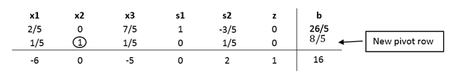
● Creating a new tableau

The new tableau will be used to identify a new possible optimal solution. Now that the pivot variable has been identified in Step 5, row operations can be performed to optimize the pivot variable while keeping the rest of the tableau equivalent.

● Checking for optimality

The optimal solution of a maximization linear programming model are the values assigned to the variables in the objective function to give the largest zeta value. Optimality will need to be checked after each new tableau to see if a new pivot variable needs to be identified. A solution is considered optimal if all values in the bottom row are greater than or equal to zero. If all values are greater than or equal to zero, the solution is considered optimal and Steps 8 through 11 can be ignored. If negative values exist, the solution is still not optimal and a new pivot point will need to be determined which is demonstrated in Step 8.

● Identify optimal values

Once the tableau is proven optimal the optimal values can be identified. These can be found by distinguishing the basic and non-basic variables. A basic variable can be classified to have a single 1 value in its column and the rest be all zeros. If a variable does not meet this criterion, it is considered non-basic. If a variable is non-basic it means the optimal solution of that variable is zero. If a variable is basic, the row that contains the 1 value will correspond to the beta value. The beta value will represent the optimal solution for the given variable.

Basic variables: x1, s1, z

Non-basic variables: x2, x3, s2

UNIT 3

Pure and MIxed Strategy

Domination

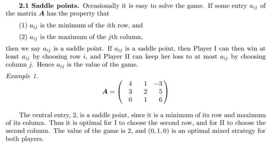
Saddle Point:

UNIT 4

Dynamic Programming

Dynamic programming is an optimization approach that transforms a complex problem into a sequence of simpler problems;

Its essential characteristic is the multistage nature of the optimization procedure.
It is a technique for getting solutions for multistage decision problems. A problem, in which the decision has to be made at successive stages, is called a multistage decision problem.
Decisions are optimized in stages rather than simultaneously
The technique of Dynamic programming was developed by Richard Bellman in early 1950.

CHARACTERISTICS OF DYNAMIC PROGRAMMING: The basic features, which characterize the dynamic programming problem, are as follows:

• The problem can be sub-divided into stages with a policy decision required at each stage. A stage is a device to sequence the decisions. That is, it decomposes a problem into sub-problems such that an optimal solution to the problem can be obtained from the optimal solution to the sub-problem.

• Every stage consists of a number of states associated with it. The states are the different possible conditions in which the system may find itself at that stage of the problem.

• Decision at each stage converts the current stage into the state associated with the next stage.

• The state of the system at a stage is described by a set of variables, called state variables.

• When the current state is known, an optimal policy for the remaining stages is independent of the policy of the previous ones.

• To identify the optimum policy for each state of the system, a recursive equation is formulated with ‘n’ stages remaining, given the optimal policy for each stage with
(n – 1) stages left.

• Using a recursive equation approach each time the solution procedure moves backward, stage by stage for obtaining the optimum policy of each stage for that particular stage, still it attains the optimum policy beginning at the initial stage.

Principle of Optimality: Bellman’s Principle

Bellman’s Principle of optimality states that ‘‘An optimal policy (a sequence of decisions) has the property that whatever the initial state and decision are, the remaining decisions must constitute an optimal policy with regard to the state resulting from the first decision.’’

This principle implies that a wrong decision taken at a stage does not prevent from making optimal decisions for the reaming stages.
This principle is the firm base for dynamic programming techniques. In light of this, we can write a recurrence relation, which enables us to make the optimal decision at each stage. Steps in getting the solution for dynamic programming problem:
The mathematical formulation of the problem and to write the recursive equation (recursive relation connecting the optimal decision function for the ‘n’ stage problem with the optimal decision function for the (n – 1) stage subproblem).
To write the relation giving the optimal decision function for one stage subproblem and solve it. • To solve the optimal decision function for 2-stage, 3-stage................ (n – 1) stage and then nstage problem.

Shortest Path using Dynamic Programming:

UNIT - 5

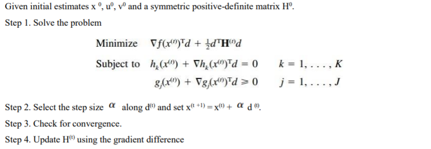
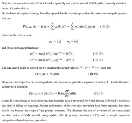
CONSTRAINED VARIABLE METRIC (CVM)

The variable metric methods have been analyzed and exploited in the past to achieve a superlinear rate of convergence in unconstrained optimization.

Recently, the update formulas used in these methods have been extended for constrained optimization.
The update formulas construct approximate second-order derivatives using first-order information.
These are referred to as constrained variable metric (CVM) methods.