Integral
FromA definite integral of a function can be represented as the signed area of the region bounded by its graph.
In , an integral assigns numbers to functions in a way that can describe displacement, area, volume, and other concepts that arise by combining data. Integration is one of the two main operations of ; its inverse operation, , is the other. Given a f of a x and an [a, b] of the , the definite integral
∫ a b f ( x ) d x {\displaystyle \int _{a}^{b}f(x)\,dx}
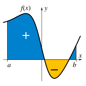
can be interpreted informally as the signed of the region in the xy-plane that is bounded by the of f, the x-axis and the vertical lines x = a and x = b. The area above the x-axis adds to the total and that below the x-axis subtracts from the total.
The operation of integration, up to an additive constant, is the inverse of the operation of differentiation. For this reason, the term integral may also refer to the related notion of the , a function F whose derivative is the given function f. In this case, it is called an indefinite integral and is written:
F ( x ) = ∫ f ( x ) d x . {\displaystyle F(x)=\int f(x)\,dx.}

The integrals discussed in this article are those termed definite integrals. It is the that connects differentiation with the definite integral: if f is a continuous real-valued function defined on a [a, b], then, once an antiderivative F of f is known, the definite integral of f over that interval is given by
∫ a b f ( x ) d x = [ F ( x ) ] a b = F ( b ) − F ( a ) . {\displaystyle \int _{a}^{b}\,f(x)dx=\left[F(x)\right]_{a}^{b}=F(b)-F(a)\,.}

The principles of integration were formulated independently by and in the late 17th century, who thought of the integral as an infinite sum of rectangles of width. gave a rigorous mathematical definition of integrals. It is based on a limiting procedure that approximates the area of a region by breaking the region into thin vertical slabs. Beginning in the 19th century, more sophisticated notions of integrals began to appear, where the type of the function as well as the over which the integration is performed has been generalised. A is defined for functions of two or more variables, and the interval of integration [a, b] is replaced by a connecting the two endpoints. In a , the curve is replaced by a piece of a in .
Pre-calculus integration[]
The first documented systematic technique capable of determining integrals is the of the astronomer (ca. 370 BC), which sought to find areas and volumes by breaking them up into an infinite number of divisions for which the area or volume was known. This method was further developed and employed by in the 3rd century BC and used to calculate the , the and of a , area of an , the area under a , the volume of a segment of a of revolution, the volume of a segment of a of revolution, and the area of a .[1]
A similar method was independently developed in China around the 3rd century AD by , who used it to find the area of the circle. This method was later used in the 5th century by Chinese father-and-son mathematicians and to find the volume of a sphere (; , pp. 125–126).
In the Middle East, Hasan Ibn al-Haytham, Latinized as (c. 965 – c. 1040 AD) derived a formula for the sum of . He used the results to carry out what would now be called an integration of this function, where the formulae for the sums of integral squares and fourth powers allowed him to calculate the volume of a .[2]
The next significant advances in integral calculus did not begin to appear until the 17th century. At this time, the work of with his , and work by , began to lay the foundations of modern calculus, with Cavalieri computing the integrals of xn up to degree n = 9 in . Further steps were made in the early 17th century by and , who provided the first hints of a connection between integration and . Barrow provided the first proof of the . generalized Cavalieri's method, computing integrals of x to a general power, including negative powers and fractional powers.
Leibniz and Newton[]
The major advance in integration came in the 17th century with the independent discovery of the by and . Leibniz published his work on calculus before Newton. The theorem demonstrates a connection between integration and differentiation. This connection, combined with the comparative ease of differentiation, can be exploited to calculate integrals. In particular, the fundamental theorem of calculus allows one to solve a much broader class of problems. Equal in importance is the comprehensive mathematical framework that both Leibniz and Newton developed. Given the name infinitesimal calculus, it allowed for precise analysis of functions within continuous domains. This framework eventually became modern , whose notation for integrals is drawn directly from the work of Leibniz.
Formalization[]
While Newton and Leibniz provided a systematic approach to integration, their work lacked a degree of . memorably attacked the vanishing increments used by Newton, calling them "". Calculus acquired a firmer footing with the development of . Integration was first rigorously formalized, using limits, by . Although all bounded piecewise continuous functions are Riemann-integrable on a bounded interval, subsequently more general functions were considered—particularly in the context of —to which Riemann's definition does not apply, and formulated a , founded in (a subfield of ). Other definitions of integral, extending Riemann's and Lebesgue's approaches, were proposed. These approaches based on the real number system are the ones most common today, but alternative approaches exist, such as a definition of integral as the of an infinite Riemann sum, based on the system.
Historical notation[]
The notation for the indefinite integral was introduced by in 1675 (, p. 359 harvnb error: no target: CITEREFBurton1988 (); , p. 154). He adapted the , ∫, from the letter ſ (), standing for summa (written as ſumma; Latin for "sum" or "total"). The modern notation for the definite integral, with limits above and below the integral sign, was first used by in Mémoires of the French Academy around 1819–20, reprinted in his book of 1822 (, pp. 249–250; , §231).
used a small vertical bar above a variable to indicate integration, or placed the variable inside a box. The vertical bar was easily confused with .x or x′, which are used to indicate differentiation, and the box notation was difficult for printers to reproduce, so these notations were not widely adopted.
First use of the term[]
The term was first printed in Latin in 1690: "Ergo et horum Integralia aequantur" (, Opera 1744, Vol. 1, p. 423)[3].
The term is used in an easy to understand paragraph from in 1696:[4]
Dans tout cela il n'y a encore que la premiere partie du calcul de M. Leibniz, laquelle consiste à descendre des grandeurs entiéres à leur différences infiniment petites, et à comparer entr'eux ces infiniment petits de quelque genre qu'ils soient: c'est ce qu'on appel calcul différentiel. Pour l'autre partie, qu'on appelle Calcul intégral, et qui consiste à remonter de ces infiniment petits aux grandeurs ou aux touts dont ils sont les différences, c'est-à-dire à en trouver les sommes, j'avois aussi dessein de le donner. Mais M. Leibniz m'ayant écrit qu'il y travailloit dans un Traité qu'il intitule De Scientia infiniti, je n'ay eu garde de prive le public d'un si bel Ouvrage qui doit renfermer tout ce qu'il y a de plus curieux pour la Méthode inverse des Tangentes...
"In all that there is still only the first part of M. Leibniz calculus, consisting in going down from integral quantities to their infinitely small differences, and in comparing between one another those infinitely smalls of any possible sort: this is what is called differential calculus. As for the other part, that is called integral calculus, and that consists in going back up from those infinitely smalls to the quantities, or the full parts to which they are the differences, that is to say to find their sums, I also had the intention to expose it. But considering M. Leibniz wrote to me that he was working on it in a book which he calls De Scientia infiniti, I took care not to deprive the public of such a beautiful work which is due to contain all what is most curious in the reverse method of the tangents..."
Integrals are used extensively in many areas of mathematics as well as in many other areas that rely on mathematics.
For example, in , integrals are used to determine the probability of some falling within a certain range. Moreover, the integral under an entire must equal 1, which provides a test of whether a with no negative values could be a density function or not.
Integrals can be used for computing the of a two-dimensional region that has a curved boundary, as well as of a three-dimensional object that has a curved boundary. The area of a two-dimensional region can be calculated using the aforementioned definite integral.
The volume of a three-dimensional object such as a disc or washer, as outlined in can be computed using the equation for the volume of a cylinder, π r 2 h {\displaystyle \pi r^{2}h} 


π ∫ a b ( − x 2 + 5 ) 2 d x {\displaystyle \pi \int _{a}^{b}(-x^{2}+5)^{2}\,dx}
The components of the above integral represent the variables in the equation for the volume of a cylinder, π r 2 h {\displaystyle \pi r^{2}h}  . The constant pi is factored out, while the radius, − x 2 + 5 {\displaystyle -x^{2}+5} , is squared within the integral. The height, represented in the volume formula by h {\displaystyle h} , is given in this integral by the infinitesimally small (in order to approximate the volume with the greatest possible accuracy) term d x {\displaystyle dx}
  .
.Integrals are also used in physics, in areas like to find quantities like , , and . For example, in rectilinear motion, the displacement of an object over the time interval [ a , b ] {\displaystyle [a,b]} 
x ( b ) − x ( a ) = ∫ a b v ( t ) d t , {\displaystyle x(b)-x(a)=\int _{a}^{b}v(t)\,dt,}

where v ( t ) {\displaystyle v(t)} 


W A → B = ∫ A B F ( x ) d x . {\displaystyle W_{A\rightarrow B}=\int _{A}^{B}F(x)\,dx.}

Integrals are also used in , where is used to calculate the difference in free energy between two given states.
Terminology and notation[]
Standard[]
The integral with respect to x of a f of a real variable x on the interval [a, b] is written as
∫ a b f ( x ) d x . {\displaystyle \int _{a}^{b}f(x)\,dx.}

The integral sign ∫ represents integration. The symbol dx, called the of the variable x, indicates that the variable of integration is x. The function f(x) to be integrated is called the integrand. The symbol dx is separated from the integrand by a space (as shown). A function is said to be integrable if the integral of the function over its domain is finite. The points a and b are called the limits of the integral. An integral where the limits are specified is called a definite integral. The integral is said to be over the interval [a, b].
If the integral goes from a finite value a to the upper limit infinity, the integral expresses the limit of the integral from a to a value b as b goes to infinity. If the value of the integral gets closer and closer to a finite value, the integral is said to to that value. If not, the integral is said to diverge.
When the limits are omitted, as in
∫ f ( x ) d x , {\displaystyle \int f(x)\,dx,}

the integral is called an indefinite integral, which represents a class of functions (the ) whose derivative is the integrand. The relates the evaluation of definite integrals to indefinite integrals. Occasionally, limits of integration are omitted for definite integrals when the same limits occur repeatedly in a particular context. Usually, the author will make this convention clear at the beginning of the relevant text.
There are several extensions of the notation for integrals to encompass integration on unbounded domains and/or in multiple dimensions (see later sections of this article).
Meaning of the symbol dx[]
Historically, the symbol dx was taken to represent an infinitesimally "small piece" of the x to be multiplied by the integrand and summed up in an infinite sense. While this notion is still heuristically useful, later mathematicians have deemed infinitesimal quantities to be untenable from the standpoint of the real number system.[5] In introductory calculus, the expression dx is therefore not assigned an independent meaning; instead, it is viewed as part of the symbol for integration and serves as its delimiter on the right side of the expression being integrated.
In more sophisticated contexts, dx can have its own significance, the meaning of which depending on the particular area of mathematics being discussed. When used in one of these ways, the original Leibnitz notation is co-opted to apply to a generalization of the original definition of the integral. Some common interpretations of dx include: an integrator function in (indicated by dα(x) in general), a in Lebesgue theory (indicated by dμ in general), or a in exterior calculus (indicated by d x i 1 ∧ ⋯ ∧ d x i k {\displaystyle dx^{i_{1}}\wedge \cdots \wedge dx^{i_{k}}} 
Conversely, in advanced settings, it is not uncommon to leave out dx when only the simple Riemann integral is being used, or the exact type of integral is immaterial. For instance, one might write ∫ a b ( c 1 f + c 2 g ) = c 1 ∫ a b f + c 2 ∫ a b g {\textstyle \int _{a}^{b}(c_{1}f+c_{2}g)=c_{1}\int _{a}^{b}f+c_{2}\int _{a}^{b}g} 
Variants[]
In , a reflected integral symbol is used instead of the symbol ∫, since the Arabic script and mathematical expressions go right to left.[6]
Some authors, particularly of European origin, use an upright "d" to indicate the variable of integration (i.e., dx instead of dx), since properly speaking, "d" is not a variable.
The symbol dx is not always placed after f(x), as for instance in
∫ 0 1 3 d x x 2 + 1 or ∫ 0 1 d x ∫ 0 1 d y e − ( x 2 + y 2 ) . {\displaystyle \int \limits _{0}^{1}{\frac {3\ dx}{x^{2}+1}}\quad {\text{ or }}\quad \int _{0}^{1}dx\int _{0}^{1}dy\ e^{-(x^{2}+y^{2})}.}

In the first expression, the differential is treated as an infinitesimal "multiplicative" factor, formally following a "commutative property" when "multiplied" by the expression 3/(x2+1). In the second expression, showing the differentials first highlights and clarifies the variables that are being integrated with respect to, a practice particularly popular with physicists.
Interpretations of the integral[]
Integrals appear in many practical situations. If a swimming pool is rectangular with a flat bottom, then from its length, width, and depth we can easily determine the volume of water it can contain (to fill it), the area of its surface (to cover it), and the length of its edge (to rope it). But if it is oval with a rounded bottom, all of these quantities call for integrals. Practical approximations may suffice for such trivial examples, but (of any discipline) requires exact and rigorous values for these elements.
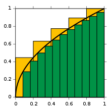
Approximations to integral of √x from 0 to 1, with 5 ■ (yellow) right endpoint partitions and 12 ■ (green) left endpoint partitions
To start off, consider the curve y = f(x) between x = 0 and x = 1 with f(x) = √x (see figure). We ask:
What is the area under the function f, in the interval from 0 to 1?
and call this (yet unknown) area the (definite) integral of f. The notation for this integral will be
∫ 0 1 x d x . {\displaystyle \int _{0}^{1}{\sqrt {x}}\ dx.}

As a first approximation, look at the unit square given by the sides x = 0 to x = 1 and y = f(0) = 0 and y = f(1) = 1. Its area is exactly 1. Actually, the true value of the integral must be somewhat less than 1. Decreasing the width of the approximation rectangles and increasing the number of rectangles gives a better result; so cross the interval in five steps, using the approximation points 0, 1/5, 2/5, and so on to 1. Fit a box for each step using the right end height of each curve piece, thus √1/5, √2/5, and so on to √1 = 1. Summing the areas of these rectangles, we get a better approximation for the sought integral, namely
1 5 ( 1 5 − 0 ) + 2 5 ( 2 5 − 1 5 ) + ⋯ + 5 5 ( 5 5 − 4 5 ) ≈ 0.7497. {\displaystyle \textstyle {\sqrt {\frac {1}{5}}}\left({\frac {1}{5}}-0\right)+{\sqrt {\frac {2}{5}}}\left({\frac {2}{5}}-{\frac {1}{5}}\right)+\cdots +{\sqrt {\frac {5}{5}}}\left({\frac {5}{5}}-{\frac {4}{5}}\right)\approx 0.7497.}

We are taking a sum of finitely many function values of f, multiplied with the differences of two subsequent approximation points. We can easily see that the approximation is still too large. Using more steps produces a closer approximation, but will always be too high and will never be exact. Alternatively, replacing these subintervals by ones with the left end height of each piece, we will get an approximation that is too low: for example, with twelve such subintervals we will get an approximate value for the area of 0.6203.
The key idea is the transition from adding finitely many differences of approximation points multiplied by their respective function values to using infinitely many fine, or steps. When this transition is completed in the above example, it turns out that the area under the curve within the stated bounds is 2/3.
The notation
∫ f ( x ) d x {\displaystyle \int f(x)\ dx}
conceives the integral as a weighted sum, denoted by the elongated s, of function values, f(x), multiplied by infinitesimal step widths, the so-called differentials, denoted by dx.
Historically, after the failure of early efforts to rigorously interpret infinitesimals, Riemann formally defined integrals as a of weighted sums, so that the dx suggested the limit of a difference (namely, the interval width). Shortcomings of Riemann's dependence on intervals and continuity motivated newer definitions, especially the , which is founded on an ability to extend the idea of "measure" in much more flexible ways. Thus the notation
∫ A f ( x ) d μ {\displaystyle \int _{A}f(x)\ d\mu }

refers to a weighted sum in which the function values are partitioned, with μ measuring the weight to be assigned to each value. Here A denotes the region of integration.
Darboux upper sums of the function y = x2
Darboux lower sums of the function y = x2
Formal definitions[]
There are many ways of formally defining an integral, not all of which are equivalent. The differences exist mostly to deal with differing special cases which may not be integrable under other definitions, but also occasionally for pedagogical reasons. The most commonly used definitions of integral are Riemann integrals and Lebesgue integrals.
Riemann integral[]
The Riemann integral is defined in terms of of functions with respect to tagged partitions of an interval. of the real line; then a tagged partition of [a, b] is a finite sequence
a = x 0 ≤ t 1 ≤ x 1 ≤ t 2 ≤ x 2 ≤ ⋯ ≤ x n − 1 ≤ t n ≤ x n = b . {\displaystyle a=x_{0}\leq t_{1}\leq x_{1}\leq t_{2}\leq x_{2}\leq \cdots \leq x_{n-1}\leq t_{n}\leq x_{n}=b.\,\!}

This partitions the interval [a, b] into n sub-intervals [xi−1, xi] indexed by i, each of which is "tagged" with a distinguished point ti ∈ [xi−1, xi]. A Riemann sum of a function f with respect to such a tagged partition is defined as
∑ i = 1 n f ( t i ) Δ i ; {\displaystyle \sum _{i=1}^{n}f(t_{i})\,\Delta _{i};}

thus each term of the sum is the area of a rectangle with height equal to the function value at the distinguished point of the given sub-interval, and width the same as the sub-interval width. Let Δi = xi−xi−1 be the width of sub-interval i; then the mesh of such a tagged partition is the width of the largest sub-interval formed by the partition, maxi=1...n Δi. The Riemann integral of a function f over the interval [a, b] is equal to S if:
For all ε > 0 there exists δ > 0 such that, for any tagged partition [a, b] with mesh less than δ, we have
| S − ∑ i = 1 n f ( t i ) Δ i | < ε . {\displaystyle \left|S-\sum _{i=1}^{n}f(t_{i})\,\Delta _{i}\right|<\varepsilon .}

When the chosen tags give the maximum (respectively, minimum) value of each interval, the Riemann sum becomes an upper (respectively, lower) , suggesting the close connection between the Riemann integral and the .
Lebesgue integral[]
Riemann–Darboux's integration (top) and Lebesgue integration (bottom)It is often of interest, both in theory and applications, to be able to pass to the limit under the integral. For instance, a sequence of functions can frequently be constructed that approximate, in a suitable sense, the solution to a problem. Then the integral of the solution function should be the limit of the integrals of the approximations. However, many functions that can be obtained as limits are not Riemann-integrable, and so such limit theorems do not hold with the Riemann integral. Therefore, it is of great importance to have a definition of the integral that allows a wider class of functions to be integrated ().
Such an integral is the Lebesgue integral, that exploits the following fact to enlarge the class of integrable functions: if the values of a function are rearranged over the domain, the integral of a function should remain the same. Thus introduced the integral bearing his name, explaining this integral thus in a letter to :
I have to pay a certain sum, which I have collected in my pocket. I take the bills and coins out of my pocket and give them to the creditor in the order I find them until I have reached the total sum. This is the Riemann integral. But I can proceed differently. After I have taken all the money out of my pocket I order the bills and coins according to identical values and then I pay the several heaps one after the other to the creditor. This is my integral.
—
Read Next page