Integral
From
If f is integrable on [a, b] then
∫ a b f ( x ) d x = F ( b ) − F ( a ) . {\displaystyle \int _{a}^{b}f(x)\,dx=F(b)-F(a).}

Calculating integrals[]
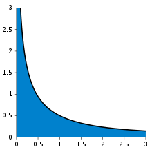
The second fundamental theorem allows many integrals to be calculated explicitly. For example, to calculate the integral
∫ 0 1 x 1 / 2 d x , {\displaystyle \int _{0}^{1}x^{1/2}\,dx,}

of the square root function f(x) = x1/2 between 0 and 1, it is sufficient to find an antiderivative, that is, a function F(x) whose derivative equals f(x):
F ′ ( x ) = f ( x ) . {\displaystyle F'(x)=f(x).}

One such function is F ( x ) = 2 3 x 3 / 2 {\displaystyle F(x)={\tfrac {2}{3}}x^{3/2}} 
∫ 0 1 x 1 / 2 d x = F ( 1 ) − F ( 0 ) = 2 3 ( 1 ) 3 / 2 − 2 3 ( 0 ) 3 / 2 = 2 3 . {\displaystyle \int _{0}^{1}x^{1/2}\,dx\ =\ F(1)-F(0)\ =\ {\tfrac {2}{3}}(1)^{3/2}-{\tfrac {2}{3}}(0)^{3/2}\ =\ {\tfrac {2}{3}}.}

This is a case of a general rule, that for f ( x ) = x q {\displaystyle f(x)=x^{q}} 


Extensions[]
Improper integrals[]
The∫ 0 ∞ d x ( x + 1 ) x = π {\displaystyle \int _{0}^{\infty }{\frac {dx}{(x+1){\sqrt {x}}}}=\pi }

has unbounded intervals for both domain and range.
A "proper" Riemann integral assumes the integrand is defined and finite on a closed and bounded interval, bracketed by the limits of integration. An improper integral occurs when one or more of these conditions is not satisfied. In some cases such integrals may be defined by considering the of a of proper on progressively larger intervals.
If the interval is unbounded, for instance at its upper end, then the improper integral is the limit as that endpoint goes to infinity.
∫ a ∞ f ( x ) d x = lim b → ∞ ∫ a b f ( x ) d x {\displaystyle \int _{a}^{\infty }f(x)\,dx=\lim _{b\to \infty }\int _{a}^{b}f(x)\,dx}

If the integrand is only defined or finite on a half-open interval, for instance (a, b], then again a limit may provide a finite result.
∫ a b f ( x ) d x = lim ε → 0 ∫ a + ϵ b f ( x ) d x {\displaystyle \int _{a}^{b}f(x)\,dx=\lim _{\varepsilon \to 0}\int _{a+\epsilon }^{b}f(x)\,dx}

That is, the improper integral is the of proper integrals as one endpoint of the interval of integration approaches either a specified , or ∞, or −∞. In more complicated cases, limits are required at both endpoints, or at interior points.
Multiple integration[]
Double integral computes volume under a surface z = f ( x , y ) {\displaystyle z=f(x,y)}
Just as the definite integral of a positive function of one variable represents the of the region between the graph of the function and the x-axis, the double integral of a positive function of two variables represents the of the region between the surface defined by the function and the plane that contains its domain. For example, a function in two dimensions depends on two real variables, x and y, and the integral of a function f over the rectangle R given as the of two intervals R = [ a , b ] × [ c , d ] {\displaystyle R=[a,b]\times [c,d]} 
∫ R f ( x , y ) d A {\displaystyle \int _{R}f(x,y)\,dA}

where the differential dA indicates that integration is taken with respect to area. This can be defined using , and represents the (signed) volume under the graph of z = f(x,y) over the domain R. Under suitable conditions (e.g., if f is continuous), states that this integral can be expressed as an equivalent iterated integral
∫ a b [ ∫ c d f ( x , y ) d y ] d x . {\displaystyle \int _{a}^{b}\left[\int _{c}^{d}f(x,y)\,dy\right]\,dx.}

This reduces the problem of computing a double integral to computing one-dimensional integrals. Because of this, another notation for the integral over R uses a double integral sign:
∬ R f ( x , y ) d A . {\displaystyle \iint _{R}f(x,y)\,dA.}
Integration over more general domains is possible. The integral of a function f, with respect to volume, over an n-dimensional region D of R n {\displaystyle \mathbb {R} ^{n}} 
∫ D f ( x ) d n x = ∫ D f d V . {\displaystyle \int _{D}f(\mathbf {x} )d^{n}\mathbf {x} \ =\int _{D}f\,dV.}

Line integrals[]
A line integral sums together elements along a curve.The concept of an integral can be extended to more general domains of integration, such as curved lines and surfaces inside higher-dimensional spaces. Such integrals are known as line integrals and surface integrals respectively. These have important applications in physics, as when dealing with .
A line integral (sometimes called a path integral) is an integral where the to be integrated is evaluated along a . Various different line integrals are in use. In the case of a closed curve it is also called a contour integral.
The function to be integrated may be a or a . The value of the line integral is the sum of values of the field at all points on the curve, weighted by some scalar function on the curve (commonly or, for a vector field, the of the vector field with a vector in the curve). This weighting distinguishes the line integral from simpler integrals defined on . Many simple formulas in physics have natural continuous analogs in terms of line integrals; for example, the fact that is equal to , F, multiplied by displacement, s, may be expressed (in terms of vector quantities) as:
W = F ⋅ s . {\displaystyle W=\mathbf {F} \cdot \mathbf {s} .}

For an object moving along a path C in a F such as an or , the total work done by the field on the object is obtained by summing up the differential work done in moving from s to s + ds. This gives the line integral
W = ∫ C F ⋅ d s . {\displaystyle W=\int _{C}\mathbf {F} \cdot d\mathbf {s} .}

Surface integrals[]
The definition of surface integral relies on splitting the surface into small surface elements.A surface integral generalizes double integrals to integration over a (which may be a curved set in ); it can be thought of as the analog of the . The function to be integrated may be a or a . The value of the surface integral is the sum of the field at all points on the surface. This can be achieved by splitting the surface into surface elements, which provide the partitioning for Riemann sums.
For an example of applications of surface integrals, consider a vector field v on a surface S; that is, for each point x in S, v(x) is a vector. Imagine that we have a fluid flowing through S, such that v(x) determines the velocity of the fluid at x. The is defined as the quantity of fluid flowing through S in unit amount of time. To find the flux, we need to take the of v with the unit to S at each point, which will give us a scalar field, which we integrate over the surface:
∫ S v ⋅ d S . {\displaystyle \int _{S}{\mathbf {v} }\cdot \,d{\mathbf {S} }.}

The fluid flux in this example may be from a physical fluid such as water or air, or from electrical or magnetic flux. Thus surface integrals have applications in physics, particularly with the of .
Contour integrals[]
In , the integrand is a of a complex variable z instead of a real function of a real variable x. When a complex function is integrated along a curve γ {\displaystyle \gamma } 
∫ γ f ( z ) d z . {\displaystyle \int _{\gamma }f(z)\,dz.}

This is known as a .
Integrals of differential forms[]
A is a mathematical concept in the fields of , , and . Differential forms are organized by degree. For example, a one-form is a weighted sum of the differentials of the coordinates, such as:
E ( x , y , z ) d x + F ( x , y , z ) d y + G ( x , y , z ) d z {\displaystyle E(x,y,z)\,dx+F(x,y,z)\,dy+G(x,y,z)\,dz}

where E, F, G are functions in three dimensions. A differential one-form can be integrated over an oriented path, and the resulting integral is just another way of writing a line integral. Here the basic differentials dx, dy, dz measure infinitesimal oriented lengths parallel to the three coordinate axes.
A differential two-form is a sum of the form
G ( x , y , z ) d x ∧ d y + E ( x , y , z ) d y ∧ d z + F ( x , y , z ) d z ∧ d x . {\displaystyle G(x,y,z)\,dx\wedge dy+E(x,y,z)\,dy\wedge dz+F(x,y,z)\,dz\wedge dx.}

Here the basic two-forms d x ∧ d y , d z ∧ d x , d y ∧ d z {\displaystyle dx\wedge dy,dz\wedge dx,dy\wedge dz} 

 .
.
Unlike the cross product, and the three-dimensional vector calculus, the wedge product and the calculus of differential forms makes sense in arbitrary dimension and on more general manifolds (curves, surfaces, and their higher-dimensional analogs). The plays the role of the and of vector calculus, and simultaneously generalizes the three theorems of vector calculus: the , , and the .
Summations[]
The discrete equivalent of integration is . Summations and integrals can be put on the same foundations using the theory of or .
Computation[]
Analytical[]
The most basic technique for computing definite integrals of one real variable is based on the . Let f(x) be the function of x to be integrated over a given interval [a, b]. Then, find an antiderivative of f; that is, a function F such that F′ = f on the interval. Provided the integrand and integral have no on the path of integration, by the fundamental theorem of calculus,
∫ a b f ( x ) d x = F ( b ) − F ( a ) . {\displaystyle \int _{a}^{b}f(x)\,dx=F(b)-F(a).}

The integral is not actually the antiderivative, but the fundamental theorem provides a way to use antiderivatives to evaluate definite integrals.
The most difficult step is usually to find the antiderivative of f. It is rarely possible to glance at a function and write down its antiderivative. More often, it is necessary to use one of the many techniques that have been developed to evaluate integrals. Most of these techniques rewrite one integral as a different one which is hopefully more tractable. Techniques include:
Alternative methods exist to compute more complex integrals. Many can be expanded in a and integrated term by term. Occasionally, the resulting infinite series can be summed analytically. The method of convolution using can also be used, assuming that the integrand can be written as a product of Meijer G-functions. There are also many less common ways of calculating definite integrals; for instance, can be used to transform an integral over a rectangular region into an infinite sum. Occasionally, an integral can be evaluated by a trick; for an example of this, see .
Computations of volumes of can usually be done with or .
Specific results which have been worked out by various techniques are collected in the .
Symbolic[]
Many problems in mathematics, physics, and engineering involve integration where an explicit formula for the integral is desired. Extensive have been compiled and published over the years for this purpose. With the spread of computers, many professionals, educators, and students have turned to that are specifically designed to perform difficult or tedious tasks, including integration. Symbolic integration has been one of the motivations for the development of the first such systems, like and .
A major mathematical difficulty in symbolic integration is that in many cases, a closed formula for the antiderivative of a rather simple-looking function does not exist. For instance, it is known that the antiderivatives of the functions exp(x2), xx and (sin x)/x cannot be expressed in the closed form involving only and functions, , and , and the operations of multiplication and composition; in other words, none of the three given functions is integrable in , which are the functions which may be built from rational functions, , logarithm, and exponential functions. The provides a general criterion to determine whether the antiderivative of an elementary function is elementary, and, if it is, to compute it. Unfortunately, it turns out that functions with closed expressions of antiderivatives are the exception rather than the rule. Consequently, computerized algebra systems have no hope of being able to find an antiderivative for a randomly constructed elementary function. On the positive side, if the 'building blocks' for antiderivatives are fixed in advance, it may be still be possible to decide whether the antiderivative of a given function can be expressed using these blocks and operations of multiplication and composition, and to find the symbolic answer whenever it exists. The , implemented in , and other , does just that for functions and antiderivatives built from rational functions, , logarithm, and exponential functions.
Some special integrands occur often enough to warrant special study. In particular, it may be useful to have, in the set of antiderivatives, the (like the , the , the , the and so on — see for more details). Extending the Risch's algorithm to include such functions is possible but challenging and has been an active research subject.
More recently a new approach has emerged, using , which are the solutions of with polynomial coefficients. Most of the elementary and special functions are D-finite, and the integral of a D-finite function is also a D-finite function. This provides an algorithm to express the antiderivative of a D-finite function as the solution of a differential equation.
This theory also allows one to compute the definite integral of a D-function as the sum of a series given by the first coefficients, and provides an algorithm to compute any coefficient.[8]
Numerical[]
Some integrals found in real applications can be computed by closed-form antiderivatives. Others are not so accommodating. Some antiderivatives do not have closed forms, some closed forms require special functions that themselves are a challenge to compute, and others are so complex that finding the exact answer is too slow. This motivates the study and application of numerical approximations of integrals. This subject, called numerical integration or numerical quadrature, arose early in the study of integration for the purpose of making hand calculations. The development of general-purpose computers made numerical integration more practical and drove a desire for improvements. The goals of numerical integration are accuracy, reliability, efficiency, and generality, and sophisticated modern methods can vastly outperform a naive method by all four measures (; ; ).
Consider, for example, the integral
∫ − 2 2 1 5 ( 1 100 ( 322 + 3 x ( 98 + x ( 37 + x ) ) ) − 24 x 1 + x 2 ) d x {\displaystyle \int _{-2}^{2}{\tfrac {1}{5}}\left({\tfrac {1}{100}}(322+3x(98+x(37+x)))-24{\frac {x}{1+x^{2}}}\right)dx}

which has the exact answer 94/25 = 3.76. (In ordinary practice, the answer is not known in advance, so an important task — not explored here — is to decide when an approximation is good enough.) A “calculus book” approach divides the integration range into, say, 16 equal pieces, and computes function values.
Spaced function values
x
−2.00
−1.50
−1.00
−0.50
0.00
0.50
1.00
1.50
2.00
f(x)
2.22800
2.45663
2.67200
2.32475
0.64400
−0.92575
−0.94000
−0.16963
0.83600
x
−1.75
−1.25
−0.75
−0.25
0.25
0.75
1.25
1.75
f(x)
2.33041
2.58562
2.62934
1.64019
−0.32444
−1.09159
−0.60387
0.31734
Numerical quadrature methods: ■ Rectangle, ■ Trapezoid, ■ Romberg, ■ Gauss
Using the left end of each piece, the sums 16 function values and multiplies by the step width, h, here 0.25, to get an approximate value of 3.94325 for the integral. The accuracy is not impressive, but calculus formally uses pieces of infinitesimal width, so initially this may seem little cause for concern. Indeed, repeatedly doubling the number of steps eventually produces an approximation of 3.76001. However, 218 pieces are required, a great computational expense for such little accuracy; and a reach for greater accuracy can force steps so small that arithmetic precision becomes an obstacle.
A better approach replaces the rectangles used in a Riemann sum with trapezoids. The is almost as easy to calculate; it sums all 17 function values, but weights the first and last by one half, and again multiplies by the step width. This immediately improves the approximation to 3.76925, which is noticeably more accurate. Furthermore, only 210 pieces are needed to achieve 3.76000, substantially less computation than the rectangle method for comparable accuracy. The idea behind the trapezoid rule, that more accurate approximations to the function yield better approximations to the integral, can be carried further. approximates the integrand by a piecewise quadratic function. Riemann sums, the trapezoid rule, and Simpson's rule are examples of a family of quadrature rules called . The degree n Newton–Cotes quadrature rule approximates the polynomial on each subinterval by a degree n polynomial. This polynomial is chosen to interpolate the values of the function on the interval. Higher degree Newton-Cotes approximations can be more accurate, but they require more function evaluations (already Simpson's rule requires twice the function evaluations of the trapezoid rule), and they can suffer from numerical inaccuracy due to . One solution to this problem is , in which the integrand is approximated by expanding it in terms of . This produces an approximation whose values never deviate far from those of the original function.
builds on the trapezoid method to great effect. First, the step lengths are halved incrementally, giving trapezoid approximations denoted by T(h0), T(h1), and so on, where hk+1 is half of hk. For each new step size, only half the new function values need to be computed; the others carry over from the previous size (as shown in the table above). But the really powerful idea is to a polynomial through the approximations, and extrapolate to T(0). With this method a numerically exact answer here requires only four pieces (five function values). The interpolating {hk,T(hk)}k = 0...2 = {(4.00,6.128), (2.00,4.352), (1.00,3.908)} is 3.76 + 0.148h2, producing the extrapolated value 3.76 at h = 0.
often requires noticeably less work for superior accuracy. In this example, it can compute the function values at just two x positions, ±2 ⁄ √3, then double each value and sum to get the numerically exact answer. The explanation for this dramatic success lies in the choice of points. Unlike Newton–Cotes rules, which interpolate the integrand at evenly spaced points, Gaussian quadrature evaluates the function at the roots of a set of . An n-point Gaussian method is exact for polynomials of degree up to 2n − 1. The function in this example is a degree 3 polynomial, plus a term that cancels because the chosen endpoints are symmetric around zero. (Cancellation also benefits the Romberg method.)
In practice, each method must use extra evaluations to ensure an error bound on an unknown function; this tends to offset some of the advantage of the pure Gaussian method, and motivates the popular . More broadly, partitions a range into pieces based on function properties, so that data points are concentrated where they are needed most.
The computation of higher-dimensional integrals (for example, volume calculations) makes important use of such alternatives as .
A calculus text is no substitute for numerical analysis, but the reverse is also true. Even the best adaptive numerical code sometimes requires a user to help with the more demanding integrals. For example, improper integrals may require a change of variable or methods that can avoid infinite function values, and known properties like symmetry and periodicity may provide critical leverage. For example, the integral ∫ 0 1 x − 1 / 2 e − x d x {\displaystyle \int _{0}^{1}x^{-1/2}e^{-x}\,dx} 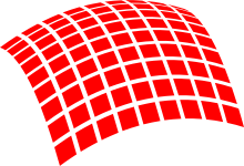 is difficult to evaluate numerically because it is infinite at x = 0. However, the substitution u = √x transforms the integral into 2 ∫ 0 1 e − u 2 d u {\displaystyle 2\int _{0}^{1}e^{-u^{2}}\,du}
Mechanical[]
The area of an arbitrary two-dimensional shape can be determined using a measuring instrument called . The volume of irregular objects can be measured with precision by the fluid as the object is submerged.
Geometrical[]
Area can sometimes be found via of an equivalent .
See also[]
- ^ Heath, Thomas Little (1897). The Works of Archimedes. England: Cambridge University Publications.
- ^ Katz, V.J. 1995. "Ideas of Calculus in Islam and India." Mathematics Magazine (Mathematical Association of America), 68(3):163–174.
- , Landmark Writings in Western Mathematics 1640-1940, Elsevier, pp. 46–58, :, 978-0-444-50871-3, retrieved 2020-07-14
- .
- was developed as a new approach to calculus that incorporates a rigorous concept of infinitesimals by using an expanded number system called the . Though placed on a sound axiomatic footing and of interest in its own right as a new area of investigation, nonstandard analysis remains somewhat controversial from a pedagogical standpoint, with proponents pointing out the intuitive nature of infinitesimals for beginning students of calculus and opponents criticizing the logical complexity of the system as a whole.
- ).
- . .
- (1967), (2nd ed.), Wiley, 978-0-471-00005-1
- (2004), Integration I, Springer Verlag, 3-540-41129-1. In particular chapters III and IV.
- Burton, David M. (2005), The History of Mathematics: An Introduction (6th ed.), McGraw-Hill, p. 359, 978-0-07-305189-5
- (1929), , Open Court Publishing, pp. 978-0-486-67766-8
- ; Björck, Åke (2008), "Chapter 5: Numerical Integration", , Philadelphia: , archived from on 2007-06-15
- Folland, Gerald B. (1984), Real Analysis: Modern Techniques and Their Applications (1st ed.), John Wiley & Sons, 978-0-471-80958-6
- (1822), , Chez Firmin Didot, père et fils, p. §231
Available in translation as Fourier, Joseph (1878), , Freeman, Alexander (trans.), Cambridge University Press, pp. 200–201 - , ed. (2002), , Dover, 978-0-486-42084-4
(Originally published by Cambridge University Press, 1897, based on J. L. Heiberg's Greek version.) - Hildebrandt, T. H. (1953), , , 59 (2): 111–139, :, 0273-0979
- Kahaner, David; ; Nash, Stephen (1989), "Chapter 5: Numerical Quadrature", , Prentice Hall, 978-0-13-627258-8
- Kallio, Bruce Victor (1966), (PDF) (M.A. thesis), University of British Columbia, archived from (PDF) on 2014-03-05, retrieved 2014-02-28
- Katz, Victor J. (2004), A History of Mathematics, Brief Version, , 978-0-321-16193-2
- (1899), Gerhardt, Karl Immanuel (ed.), , Berlin: Mayer & Müller
- ; (2001), Analysis, , 14 (2nd ed.), , 978-0821827833
- Miller, Jeff, , retrieved 2009-11-22
- O’Connor, J. J.; Robertson, E. F. (1996), , retrieved 2007-07-09
- (1987), "Chapter 1: Abstract Integration", Real and Complex Analysis (International ed.), McGraw-Hill, 978-0-07-100276-9
- (1964), (English translation by L. C. Young. With two additional notes by Stefan Banach. Second revised ed.), New York: Dover
- Shea, Marilyn (May 2007), , University of Maine, retrieved 9 January 2009
- Siegmund-Schultze, Reinhard (2008), "Henri Lebesgue", in Timothy Gowers; June Barrow-Green; Imre Leader (eds.), Princeton Companion to Mathematics, Princeton University Press.
- Stoer, Josef; Bulirsch, Roland (2002), "Topics in Integration", Introduction to Numerical Analysis (3rd ed.), Springer, 978-0-387-95452-3.
- W3C (2006),
- Keisler, H. Jerome, , University of Wisconsin
- Stroyan, K. D., , University of Iowa
- Mauch, Sean, , CIT, an online textbook that includes a complete introduction to calculus
- Crowell, Benjamin, , Fullerton College, an online textbook
- Garrett, Paul,
- Hussain, Faraz, , an online textbook
- Johnson, William Woolsey (1909) , link from .
- Kowalk, W. P., , University of Oldenburg. A new concept to an old problem. Online textbook
- Sloughter, Dan, , an introduction to calculus
- at Holistic Numerical Methods Institute
- P. S. Wang, (1972) — a cookbook of definite integral techniques