Calculus
FromCalculus equations written on a chalkboard for students
Calculus, originally called infinitesimal calculus or "the calculus of ", is the study of continuous change, in the same way that is the study of shape and is the study of generalizations of .
It has two major branches, and ; the former concerns instantaneous rates of change, and the slopes of curves, while integral calculus concerns accumulation of quantities, and areas under or between curves. These two branches are related to each other by the , and they make use of the fundamental notions of of and to a well-defined .[1]
Infinitesimal calculus was developed independently in the late 17th century by and . Today, calculus has widespread uses in , , and .[4]
In , calculus denotes courses of elementary , which are mainly devoted to the study of and limits. The word calculus (plural calculi) is a word, meaning originally "small pebble" (this meaning is ). Because such pebbles were used for calculation, the meaning of the word has evolved and today usually means a method of computation. It is therefore used for naming specific methods of calculation and related theories, such as , , , , and .
Modern calculus was developed in 17th-century Europe by and (independently of each other, first publishing around the same time) but elements of it appeared in ancient Greece, then in China and the Middle East, and still later again in medieval Europe and in India.
Ancient
The ancient period introduced some of the ideas that led to calculus, but does not seem to have developed these ideas in a rigorous and systematic way. Calculations of and , one goal of integral calculus, can be found in the (, c. 1820 BC); but the formulas are simple instructions, with no indication as to method, and some of them lack major components.[5]
From the age of , (c. 408–355 BC) used the , which foreshadows the concept of the limit, to calculate areas and volumes, while (c. 287–212 BC) , inventing which resemble the methods of integral calculus.[6]
The method of exhaustion was later discovered independently in by in the 3rd century AD in order to find the area of a circle., son of , established a method that would later be called to find the volume of a .
Medieval
Alhazen, 11th century Arab mathematician and physicist
In the Middle East, Hasan Ibn al-Haytham, Latinized as (c. 965 – c. 1040 CE) derived a formula for the sum of . He used the results to carry out what would now be called an of this function, where the formulae for the sums of integral squares and fourth powers allowed him to calculate the volume of a .[10]
In the 14th century, Indian mathematicians gave a non-rigorous method, resembling differentiation, applicable to some trigonometric functions. and the thereby stated components of calculus. A complete theory encompassing these components is now well known in the Western world as the or approximations. and the , show the connection between the two, and turn calculus into the great problem-solving tool we have today".[10]
Modern
The calculus was the first achievement of modern mathematics and it is difficult to overestimate its importance. I think it defines more unequivocally than anything else the inception of modern mathematics, and the system of mathematical analysis, which is its logical development, still constitutes the greatest technical advance in exact thinking.
—[12]
In Europe, the foundational work was a treatise written by , who argued that volumes and areas should be computed as the sums of the volumes and areas of infinitesimally thin cross-sections. The ideas were similar to Archimedes' in , but this treatise is believed to have been lost in the 13th century, and was only rediscovered in the early 20th century, and so would have been unknown to Cavalieri. Cavalieri's work was not well respected since his methods could lead to erroneous results, and the infinitesimal quantities he introduced were disreputable at first.
The formal study of calculus brought together Cavalieri's infinitesimals with the developed in Europe at around the same time. , claiming that he borrowed from , introduced the concept of , which represented equality up to an infinitesimal error term., , and , the latter two proving the around 1670.
The and , and ,[] were used by in an idiosyncratic notation which he applied to solve problems of . In his works, Newton rephrased his ideas to suit the mathematical idiom of the time, replacing calculations with infinitesimals by equivalent geometrical arguments which were considered beyond reproach. He used the methods of calculus to solve the problem of planetary motion, the shape of the surface of a rotating fluid, the oblateness of the earth, the motion of a weight sliding on a , and many other problems discussed in his (1687). In other work, he developed series expansions for functions, including fractional and irrational powers, and it was clear that he understood the principles of the . He did not publish all these discoveries, and at this time infinitesimal methods were still considered disreputable.
These ideas were arranged into a true calculus of infinitesimals by , who was originally accused of by Newton. of and contributor to calculus. His contribution was to provide a clear set of rules for working with infinitesimal quantities, allowing the computation of second and higher derivatives, and providing the and , in their differential and integral forms. Unlike Newton, Leibniz paid a lot of attention to the formalism, often spending days determining appropriate symbols for concepts.
Today, and are usually both given credit for independently inventing and developing calculus. Newton was the first to apply calculus to general and Leibniz developed much of the notation used in calculus today. The basic insights that both Newton and Leibniz provided were the laws of differentiation and integration, second and higher derivatives, and the notion of an approximating polynomial series. By Newton's time, the fundamental theorem of calculus was known.
When Newton and Leibniz first published their results, there was over which mathematician (and therefore which country) deserved credit. Newton derived his results first (later to be published in his ), but Leibniz published his "" first. Newton claimed Leibniz stole ideas from his unpublished notes, which Newton had shared with a few members of the . This controversy divided English-speaking mathematicians from continental European mathematicians for many years, to the detriment of English mathematics.[] A careful examination of the papers of Leibniz and Newton shows that they arrived at their results independently, with Leibniz starting first with integration and Newton with differentiation. It is Leibniz, however, who gave the new discipline its name. Newton called his calculus "".
Since the time of Leibniz and Newton, many mathematicians have contributed to the continuing development of calculus. One of the first and most complete works on both infinitesimal and was written in 1748 by .
Foundations
In calculus, foundations refers to the development of the subject from and definitions. In early calculus the use of quantities was thought unrigorous, and was fiercely criticized by a number of authors, most notably and . Berkeley famously described infinitesimals as the in his book in 1734. Working out a rigorous foundation for calculus occupied mathematicians for much of the century following Newton and Leibniz, and is still to some extent an active area of research today.
Several mathematicians, including , tried to prove the soundness of using infinitesimals, but it would not be until 150 years later when, due to the work of and , a way was finally found to avoid mere "notions" of infinitely small quantities., we find a broad range of foundational approaches, including a definition of in terms of infinitesimals, and a (somewhat imprecise) prototype of an in the definition of differentiation. and eliminated infinitesimals (although his definition can actually validate infinitesimals). Following the work of Weierstrass, it eventually became common to base calculus on limits instead of infinitesimal quantities, though the subject is still occasionally called "infinitesimal calculus". used these ideas to give a precise definition of the integral. It was also during this period that the ideas of calculus were generalized to and the .
In modern mathematics, the foundations of calculus are included in the field of , which contains full definitions and of the theorems of calculus. The reach of calculus has also been greatly extended. invented and used it to define integrals of all but the most functions. introduced , which can be used to take the derivative of any function whatsoever.
Limits are not the only rigorous approach to the foundation of calculus. Another way is to use 's . Robinson's approach, developed in the 1960s, uses technical machinery from to augment the real number system with and numbers, as in the original Newton-Leibniz conception. The resulting numbers are called , and they can be used to give a Leibniz-like development of the usual rules of calculus. There is also , which differs from non-standard analysis in that it mandates neglecting higher power infinitesimals during derivations.
Significance
While many of the ideas of calculus had been developed earlier in , , , , and , the use of calculus began in Europe, during the 17th century, when and built on the work of earlier mathematicians to introduce its basic principles. The development of calculus was built on earlier concepts of instantaneous motion and area underneath curves.
Applications of differential calculus include computations involving and , the of a curve, and . Applications of integral calculus include computations involving area, , , , , and . More advanced applications include and .
Calculus is also used to gain a more precise understanding of the nature of space, time, and motion. For centuries, mathematicians and philosophers wrestled with paradoxes involving or sums of infinitely many numbers. These questions arise in the study of and area. The philosopher gave several famous examples of such . Calculus provides tools, especially the and the , that resolve the paradoxes.
Principles
Limits and infinitesimals
Calculus is usually developed by working with very small quantities. Historically, the first method of doing so was by . These are objects which can be treated like real numbers but which are, in some sense, "infinitely small". For example, an infinitesimal number could be greater than 0, but less than any number in the sequence 1, 1/2, 1/3, ... and thus less than any positive . From this point of view, calculus is a collection of techniques for manipulating infinitesimals. The symbols d x {\displaystyle dx}  and d y {\displaystyle dy}
  were taken to be infinitesimal, and the derivative d y / d x {\displaystyle dy/dx}
  was simply their ratio.
The infinitesimal approach fell out of favor in the 19th century because it was difficult to make the notion of an infinitesimal precise. However, the concept was revived in the 20th century with the introduction of and , which provided solid foundations for the manipulation of infinitesimals.
In the late 19th century, infinitesimals were replaced within academia by the approach to . Limits describe the value of a at a certain input in terms of its values at nearby inputs. They capture small-scale behavior in the context of the . In this treatment, calculus is a collection of techniques for manipulating certain limits. Infinitesimals get replaced by very small numbers, and the infinitely small behavior of the function is found by taking the limiting behavior for smaller and smaller numbers. Limits were thought to provide a more rigorous foundation for calculus, and for this reason they became the standard approach during the twentieth century.
Differential calculus
Tangent line at (x, f(x)). The derivative f′(x) of a curve at a point is the slope (rise over run) of the line tangent to that curve at that point.Differential calculus is the study of the definition, properties, and applications of the of a function. The process of finding the derivative is called differentiation. Given a function and a point in the domain, the derivative at that point is a way of encoding the small-scale behavior of the function near that point. By finding the derivative of a function at every point in its domain, it is possible to produce a new function, called the derivative function or just the derivative of the original function. In formal terms, the derivative is a which takes a function as its input and produces a second function as its output. This is more abstract than many of the processes studied in elementary algebra, where functions usually input a number and output another number. For example, if the doubling function is given the input three, then it outputs six, and if the squaring function is given the input three, then it outputs nine. The derivative, however, can take the squaring function as an input. This means that the derivative takes all the information of the squaring function—such as that two is sent to four, three is sent to nine, four is sent to sixteen, and so on—and uses this information to produce another function. The function produced by deriving the squaring function turns out to be the doubling function.
In more explicit terms the "doubling function" may be denoted by g(x) = 2x and the "squaring function" by f(x) = x2. The "derivative" now takes the function f(x), defined by the expression "x2", as an input, that is all the information—such as that two is sent to four, three is sent to nine, four is sent to sixteen, and so on—and uses this information to output another function, the function g(x) = 2x, as will turn out.
The most common symbol for a derivative is an -like mark called . Thus, the derivative of a function called f is denoted by f′, pronounced "f prime". For instance, if f(x) = x2 is the squaring function, then f′(x) = 2x is its derivative (the doubling function g from above). This notation is known as .
If the input of the function represents time, then the derivative represents change with respect to time. For example, if f is a function that takes a time as input and gives the position of a ball at that time as output, then the derivative of f is how the position is changing in time, that is, it is the of the ball.
If a function is (that is, if the of the function is a straight line), then the function can be written as y = mx + b, where x is the independent variable, y is the dependent variable, b is the y-intercept, and:
m = rise run = change in y change in x = Δ y Δ x . {\displaystyle m={\frac {\text{rise}}{\text{run}}}={\frac {{\text{change in }}y}{{\text{change in }}x}}={\frac {\Delta y}{\Delta x}}.}

This gives an exact value for the slope of a straight line. If the graph of the function is not a straight line, however, then the change in y divided by the change in x varies. Derivatives give an exact meaning to the notion of change in output with respect to change in input. To be concrete, let f be a function, and fix a point a in the domain of f. (a, f(a)) is a point on the graph of the function. If h is a number close to zero, then a + h is a number close to a. Therefore, (a + h, f(a + h)) is close to (a, f(a)). The slope between these two points is
m = f ( a + h ) − f ( a ) ( a + h ) − a = f ( a + h ) − f ( a ) h . {\displaystyle m={\frac {f(a+h)-f(a)}{(a+h)-a}}={\frac {f(a+h)-f(a)}{h}}.}

This expression is called a . A line through two points on a curve is called a secant line, so m is the slope of the secant line between (a, f(a)) and (a + h, f(a + h)). The secant line is only an approximation to the behavior of the function at the point a because it does not account for what happens between a and a + h. It is not possible to discover the behavior at a by setting h to zero because this would require , which is undefined. The derivative is defined by taking the as h tends to zero, meaning that it considers the behavior of f for all small values of h and extracts a consistent value for the case when h equals zero:
lim h → 0 f ( a + h ) − f ( a ) h . {\displaystyle \lim _{h\to 0}{f(a+h)-f(a) \over {h}}.}

Geometrically, the derivative is the slope of the to the graph of f at a. The tangent line is a limit of secant lines just as the derivative is a limit of difference quotients. For this reason, the derivative is sometimes called the slope of the function f.
Here is a particular example, the derivative of the squaring function at the input 3. Let f(x) = x2 be the squaring function.
The derivative f′(x) of a curve at a point is the slope of the line tangent to that curve at that point. This slope is determined by considering the limiting value of the slopes of secant lines. Here the function involved (drawn in red) is f(x) = x3 − x. The tangent line (in green) which passes through the point (−3/2, −15/8) has a slope of 23/4. Note that the vertical and horizontal scales in this image are different.
f ′ ( 3 ) = lim h → 0 ( 3 + h ) 2 − 3 2 h = lim h → 0 9 + 6 h + h 2 − 9 h = lim h → 0 6 h + h 2 h = lim h → 0 ( 6 + h ) = 6 {\displaystyle {\begin{aligned}f'(3)&=\lim _{h\to 0}{(3+h)^{2}-3^{2} \over {h}}\\&=\lim _{h\to 0}{9+6h+h^{2}-9 \over {h}}\\&=\lim _{h\to 0}{6h+h^{2} \over {h}}\\&=\lim _{h\to 0}(6+h)\\&=6\end{aligned}}}

The slope of the tangent line to the squaring function at the point (3, 9) is 6, that is to say, it is going up six times as fast as it is going to the right. The limit process just described can be performed for any point in the domain of the squaring function. This defines the derivative function of the squaring function, or just the derivative of the squaring function for short. A computation similar to the one above shows that the derivative of the squaring function is the doubling function.
Leibniz notation
A common notation, introduced by Leibniz, for the derivative in the example above is
y = x 2 d y d x = 2 x . {\displaystyle {\begin{aligned}y&=x^{2}\\{\frac {dy}{dx}}&=2x.\end{aligned}}}

In an approach based on limits, the symbol dy/dx is to be interpreted not as the quotient of two numbers but as a shorthand for the limit computed above. Leibniz, however, did intend it to represent the quotient of two infinitesimally small numbers, dy being the infinitesimally small change in y caused by an infinitesimally small change dx applied to x. We can also think of d/dx as a differentiation operator, which takes a function as an input and gives another function, the derivative, as the output. For example:
d d x ( x 2 ) = 2 x . {\displaystyle {\frac {d}{dx}}(x^{2})=2x.}

In this usage, the dx in the denominator is read as "with respect to x". Another example of correct notation could be:
g ( t ) = t 2 + 2 t + 4 d d t g ( t ) = 2 t + 2 {\displaystyle {\begin{aligned}g(t)=t^{2}+2t+4\\\\{d \over dt}g(t)=2t+2\end{aligned}}}

Even when calculus is developed using limits rather than infinitesimals, it is common to manipulate symbols like dx and dy as if they were real numbers; although it is possible to avoid such manipulations, they are sometimes notationally convenient in expressing operations such as the .
Integral calculus
Integral calculus is the study of the definitions, properties, and applications of two related concepts, the indefinite integral and the definite integral. The process of finding the value of an integral is called integration. In technical language, integral calculus studies two related .
The indefinite integral, also known as the , is the inverse operation to the derivative. F is an indefinite integral of f when f is a derivative of F. (This use of lower- and upper-case letters for a function and its indefinite integral is common in calculus.)
The definite integral inputs a function and outputs a number, which gives the algebraic sum of areas between the graph of the input and the . The technical definition of the definite integral involves the of a sum of areas of rectangles, called a .
A motivating example is the distances traveled in a given time.
D i s t a n c e = S p e e d ⋅ T i m e {\displaystyle \mathrm {Distance} =\mathrm {Speed} \cdot \mathrm {Time} }

If the speed is constant, only multiplication is needed, but if the speed changes, a more powerful method of finding the distance is necessary. One such method is to approximate the distance traveled by breaking up the time into many short intervals of time, then multiplying the time elapsed in each interval by one of the speeds in that interval, and then taking the sum (a ) of the approximate distance traveled in each interval. The basic idea is that if only a short time elapses, then the speed will stay more or less the same. However, a Riemann sum only gives an approximation of the distance traveled. We must take the limit of all such Riemann sums to find the exact distance traveled.
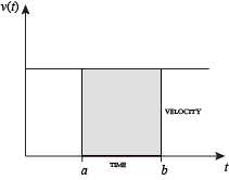
Integration can be thought of as measuring the area under a curve, defined by f(x), between two points (here a and b).
When velocity is constant, the total distance traveled over the given time interval can be computed by multiplying velocity and time. For example, travelling a steady 50 mph for 3 hours results in a total distance of 150 miles. In the diagram on the left, when constant velocity and time are graphed, these two values form a rectangle with height equal to the velocity and width equal to the time elapsed. Therefore, the product of velocity and time also calculates the rectangular area under the (constant) velocity curve. This connection between the area under a curve and distance traveled can be extended to any irregularly shaped region exhibiting a fluctuating velocity over a given time period. If f(x) in the diagram on the right represents speed as it varies over time, the distance traveled (between the times represented by a and b) is the area of the shaded region s.
To approximate that area, an intuitive method would be to divide up the distance between a and b into a number of equal segments, the length of each segment represented by the symbol Δx. For each small segment, we can choose one value of the function f(x). Call that value h. Then the area of the rectangle with base Δx and height h gives the distance (time Δx multiplied by speed h) traveled in that segment. Associated with each segment is the average value of the function above it, f(x) = h. The sum of all such rectangles gives an approximation of the area between the axis and the curve, which is an approximation of the total distance traveled. A smaller value for Δx will give more rectangles and in most cases a better approximation, but for an exact answer we need to take a limit as Δx approaches zero.
The symbol of integration is ∫ {\displaystyle \int } 
∫ a b f ( x ) d x . {\displaystyle \int _{a}^{b}f(x)\,dx.}

and is read "the integral from a to b of f-of-x with respect to x." The Leibniz notation dx is intended to suggest dividing the area under the curve into an infinite number of rectangles, so that their width Δx becomes the infinitesimally small dx. In a formulation of the calculus based on limits, the notation
∫ a b ⋯ d x {\displaystyle \int _{a}^{b}\cdots \,dx}

is to be understood as an operator that takes a function as an input and gives a number, the area, as an output. The terminating differential, dx, is not a number, and is not being multiplied by f(x), although, serving as a reminder of the Δx limit definition, it can be treated as such in symbolic manipulations of the integral. Formally, the differential indicates the variable over which the function is integrated and serves as a closing bracket for the integration operator.
The indefinite integral, or antiderivative, is written:
∫ f ( x ) d x . {\displaystyle \int f(x)\,dx.}

Functions differing by only a constant have the same derivative, and it can be shown that the antiderivative of a given function is actually a family of functions differing only by a constant. Since the derivative of the function y = x2 + C, where C is any constant, is y′ = 2x, the antiderivative of the latter is given by:
∫ 2 x d x = x 2 + C . {\displaystyle \int 2x\,dx=x^{2}+C.}

The unspecified constant C present in the indefinite integral or antiderivative is known as the .
Fundamental theorem
The states that differentiation and integration are inverse operations. More precisely, it relates the values of antiderivatives to definite integrals. Because it is usually easier to compute an antiderivative than to apply the definition of a definite integral, the fundamental theorem of calculus provides a practical way of computing definite integrals. It can also be interpreted as a precise statement of the fact that differentiation is the inverse of integration.
The fundamental theorem of calculus states: If a function f is on the interval [a, b] and if F is a function whose derivative is f on the interval (a, b), then
∫ a b f ( x ) d x = F ( b ) − F ( a ) . {\displaystyle \int _{a}^{b}f(x)\,dx=F(b)-F(a).}
Furthermore, for every x in the interval (a, b),
d d x ∫ a x f ( t ) d t = f ( x ) . {\displaystyle {\frac {d}{dx}}\int _{a}^{x}f(t)\,dt=f(x).}

This realization, made by both and , who based their results on earlier work by , was key to the proliferation of analytic results after their work became known. The fundamental theorem provides an algebraic method of computing many definite integrals—without performing limit processes—by finding formulas for . It is also a prototype solution of a . Differential equations relate an unknown function to its derivatives, and are ubiquitous in the sciences.
Applications
Calculus is used in every branch of the physical sciences, , , , , , , , , and in other fields wherever a problem can be and an solution is desired. It allows one to go from (non-constant) rates of change to the total change or vice versa, and many times in studying a problem we know one and are trying to find the other.
makes particular use of calculus; all concepts in and are related through calculus. The of an object of known , the of objects, as well as the total energy of an object within a conservative field can be found by the use of calculus. An example of the use of calculus in mechanics is : historically stated it expressly uses the term "change of motion" which implies the derivative saying The change of momentum of a body is equal to the resultant force acting on the body and is in the same direction. Commonly expressed today as Force = Mass × acceleration, it implies differential calculus because acceleration is the time derivative of velocity or second time derivative of trajectory or spatial position. Starting from knowing how an object is accelerating, we use calculus to derive its path.
Maxwell's theory of and 's theory of are also expressed in the language of differential calculus. Chemistry also uses calculus in determining reaction rates and radioactive decay. In biology, population dynamics starts with reproduction and death rates to model population changes.
Calculus can be used in conjunction with other mathematical disciplines. For example, it can be used with to find the "best fit" linear approximation for a set of points in a domain. Or it can be used in to determine the probability of a continuous random variable from an assumed density function. In , the study of graphs of functions, calculus is used to find high points and low points (maxima and minima), slope, and .
, which gives the relationship between a line integral around a simple closed curve C and a double integral over the plane region D bounded by C, is applied in an instrument known as a , which is used to calculate the area of a flat surface on a drawing. For example, it can be used to calculate the amount of area taken up by an irregularly shaped flower bed or swimming pool when designing the layout of a piece of property.
, which gives the relationship between a double integral of a function around a simple closed rectangular curve C and a linear combination of the antiderivative's values at corner points along the edge of the curve, allows fast calculation of sums of values in rectangular domains. For example, it can be used to efficiently calculate sums of rectangular domains in images, in order to rapidly extract features and detect object; another algorithm that could be used is the .
In the realm of medicine, calculus can be used to find the optimal branching angle of a blood vessel so as to maximize flow. From the decay laws for a particular drug's elimination from the body, it is used to derive dosing laws. In nuclear medicine, it is used to build models of radiation transport in targeted tumor therapies.
In economics, calculus allows for the determination of maximal profit by providing a way to easily calculate both and .
Calculus is also used to find approximate solutions to equations; in practice it is the standard way to solve differential equations and do root finding in most applications. Examples are methods such as , , and . For instance, spacecraft use a variation of the to approximate curved courses within zero gravity environments.
Varieties
Over the years, many reformulations of calculus have been investigated for different purposes.
Non-standard calculus
Imprecise calculations with infinitesimals were widely replaced with the rigorous starting in the 1870s. Meanwhile, calculations with infinitesimals persisted and often led to correct results. This led to investigate if it were possible to develop a number system with infinitesimal quantities over which the theorems of calculus were still valid. In 1960, building upon the work of and , he succeeded in developing . The theory of non-standard analysis is rich enough to be applied in many branches of mathematics. As such, books and articles dedicated solely to the traditional theorems of calculus often go by the title .
Smooth infinitesimal analysis
This is another reformulation of the calculus in terms of . Based on the ideas of and employing the methods of , it views all functions as being and incapable of being expressed in terms of entities. One aspect of this formulation is that the does not hold in this formulation.
Constructive analysis
is a branch of mathematics that insists that proofs of the existence of a number, function, or other mathematical object should give a construction of the object. As such constructive mathematics also rejects the . Reformulations of calculus in a constructive framework are generally part of the subject of .
See also
Lists
References- 527896.
- (1959). . New York: Dover. 643872.
- 1-56025-706-7.
- .
- , Vol. I
- 978-0-521-66160-7
- . Chinese studies in the history and philosophy of science and technology. 130. Springer. p. 279.
- 978-0-321-38700-4.
- (3 ed.). Jones & Bartlett Learning. p. xxvii.
- ^ Katz, V.J. 1995. "Ideas of Calculus in Islam and India." Mathematics Magazine (Mathematical Association of America), 68(3):163–174.
- .
- 981-02-2201-7, pp. 618–626.
- : Number theory: An approach through History from Hammurapi to Legendre. Boston: Birkhauser Boston, 1984, 0-8176-4565-9, p. 28.
- (Illustrated ed.). Springer Science & Business Media. p. 248. 978-1-931914-59-8.
- (Illustrated ed.). Springer Science & Business Media. p. 87. 978-0-387-73468-2.
- . By Cupillari, Antonella (illustrated ed.). Edwin Mellen Press. p. iii. 978-0-7734-5226-8.
- . .
- (1946). . London: . p. 857. The great mathematicians of the seventeenth century were optimistic and anxious for quick results; consequently they left the foundations of analytical geometry and the infinitesimal calculus insecure. Leibniz believed in actual infinitesimals, but although this belief suited his metaphysics it had no sound basis in mathematics. Weierstrass, soon after the middle of the nineteenth century, showed how to establish the calculus without infinitesimals, and thus at last made it logically secure. Next came Georg Cantor, who developed the theory of continuity and infinite number. "Continuity" had been, until he defined it, a vague word, convenient for philosophers like Hegel, who wished to introduce metaphysical muddles into mathematics. Cantor gave a precise significance to the word, and showed that continuity, as he defined it, was the concept needed by mathematicians and physicists. By this means a great deal of mysticism, such as that of Bergson, was rendered antiquated.
- . Cambridge: MIT Press. 978-0-387-90527-3.
Further reading
Books
- (1949). . Hafner. Dover edition 1959, 0-486-60509-4
- 978-3-540-65058-4 Introduction to calculus and analysis 1.
- . .
- Robert A. Adams. (1999). 978-0-201-39607-2 Calculus: A complete course.
- Albers, Donald J.; Richard D. Anderson and Don O. Loftsgaarden, ed. (1986) Undergraduate Programs in the Mathematics and Computer Sciences: The 1985–1986 Survey, Mathematical Association of America No. 7.
- : A Primer of Infinitesimal Analysis, Cambridge University Press, 1998. and nilpotent infinitesimals.
- , "The History of Notations of the Calculus." Annals of Mathematics, 2nd Ser., Vol. 25, No. 1 (Sep. 1923), pp. 1–46.
- Leonid P. Lebedev and Michael J. Cloud: "Approximating Perfection: a Mathematician's Journey into the World of Mechanics, Ch. 1: The Tools of Calculus", Princeton Univ. Press, 2004.
- . (2003). 978-0-471-26987-8 Calculus and Pizza: A Math Cookbook for the Hungry Mind.
- . (September 1994). 978-0-914098-89-8 Calculus. Publish or Perish publishing.
- . (1967). 978-0-471-00005-1 Calculus, Volume 1, One-Variable Calculus with an Introduction to Linear Algebra. Wiley.
- . (1969). 978-0-471-00007-5 Calculus, Volume 2, Multi-Variable Calculus and Linear Algebra with Applications. Wiley.
- and . (1998). 978-0-312-18548-0 Calculus Made Easy.
- . (1988). Calculus for a New Century; A Pump, Not a Filter, The Association, Stony Brook, NY. ED 300 252.
- Thomas/Finney. (1996). 978-0-201-53174-9 Calculus and Analytic geometry 9th, Addison Wesley.
- Weisstein, Eric W. From MathWorld—A Wolfram Web Resource.
- Howard Anton, Irl Bivens, Stephen Davis:"Calculus", John Willey and Sons Pte. Ltd., 2002. 978-81-265-1259-1
- , Bruce H. Edwards (2010). Calculus, 9th ed., Brooks Cole Cengage Learning. 978-0-547-16702-2
- McQuarrie, Donald A. (2003). Mathematical Methods for Scientists and Engineers, University Science Books. 978-1-891389-24-5
- Salas, Saturnino L.; ; Etgen, Garret J. (2007). Calculus: One and Several Variables (10th ed.). . 978-0-471-69804-3.
- (2012). Calculus: Early Transcendentals, 7th ed., Brooks Cole Cengage Learning. 978-0-538-49790-9
- , Maurice D. Weir, , Frank R. Giordano (2008), Calculus, 11th ed., Addison-Wesley.
- Boelkins, M. (2012). (PDF). Archived from on 30 May 2013. Retrieved 1 February 2013.
- Crowell, B. (2003). "Calculus". Light and Matter, Fullerton. Retrieved 6 May 2007 from
- Garrett, P. (2006). "Notes on first year calculus". University of Minnesota. Retrieved 6 May 2007 from
- Faraz, H. (2006). "Understanding Calculus". Retrieved 6 May 2007 from UnderstandingCalculus.com, URL (HTML only)
- Keisler, H.J. (2000). "Elementary Calculus: An Approach Using Infinitesimals". Retrieved 29 August 2010 from
- Mauch, S. (2004). "Sean's Applied Math Book" (pdf). California Institute of Technology. Retrieved 6 May 2007 from
- Sloughter, Dan (2000). "Difference Equations to Differential Equations: An introduction to calculus". Retrieved 17 March 2009 from
- Stroyan, K.D. (2004). "A brief introduction to infinitesimal calculus". University of Iowa. Retrieved 6 May 2007 from (HTML only)
- Strang, G. (1991). "Calculus" Massachusetts Institute of Technology. Retrieved 6 May 2007 from
- Smith, William V. (2001). "The Calculus". Retrieved 4 July 2008 [1] (HTML only).