Integral

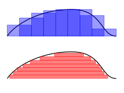
As , p. 56) puts it, "To compute the Riemann integral of f, one partitions the domain [a, b] into subintervals", while in the Lebesgue integral, "one is in effect partitioning the range of f ". The definition of the Lebesgue integral thus begins with a , μ. In the simplest case, the μ(A) of an interval A = [a, b] is its width, b − a, so that the Lebesgue integral agrees with the (proper) Riemann integral when both exist. In more complicated cases, the sets being measured can be highly fragmented, with no continuity and no resemblance to intervals.

Using the "partitioning the range of f " philosophy, the integral of a non-negative function f : R → R should be the sum over t of the areas between a thin horizontal strip between y = t and y = t + dt. This area is just μ{ x : f(x) > t} dt. Let f∗(t) = μ{ x : f(x) > t}. The Lebesgue integral of f is then defined by ()

where the integral on the right is an ordinary improper Riemann integral (f∗ is a strictly decreasing positive function, and therefore has a improper Riemann integral). For a suitable class of functions (the ) this defines the Lebesgue integral.

A general measurable function f is Lebesgue-integrable if the sum of the absolute values of the areas of the regions between the graph of f and the x-axis is finite:

In that case, the integral is, as in the Riemannian case, the difference between the area above the x-axis and the area below the x-axis:

where

Other integrals[]

Although the Riemann and Lebesgue integrals are the most widely used definitions of the integral, a number of others exist, including:

• The , which is defined by Darboux sums (restricted Riemann sums) yet is equivalent to the - a function is Darboux-integrable if and only if it is Riemann-integrable. Darboux integrals have the advantage of being easier to define than Riemann integrals.


• The , an extension of the Riemann integral which integrates with respect to a function as opposed to a variable.


• The , further developed by , which generalizes both the Riemann–Stieltjes and Lebesgue integrals.


• The , which subsumes the Lebesgue integral and without depending on .


• The , used for integration on locally compact topological groups, introduced by in 1933.


• The , variously defined by , , and (most elegantly, as the gauge integral) , and developed by .


• The and , which define integration with respect to such as .


• The , which is a kind of Riemann–Stieltjes integral with respect to certain functions of .


• The integral, which is defined for functions equipped with some additional "rough path" structure and generalizes stochastic integration against both and processes such as the .


• The , a subadditive or superadditive integral created by the French mathematician Gustave Choquet in 1953.

Linearity[]

The collection of Riemann-integrable functions on a closed interval [a, b] forms a under the operations of and multiplication by a scalar, and the operation of integration

is a on this vector space. Thus, firstly, the collection of integrable functions is closed under taking ; and, secondly, the integral of a linear combination is the linear combination of the integrals,

Similarly, the set of -valued Lebesgue-integrable functions on a given E with measure μ is closed under taking linear combinations and hence form a vector space, and the Lebesgue integral

is a linear functional on this vector space, so that

More generally, consider the vector space of all on a measure space (E,μ), taking values in a V over a locally compact K, f : E → V. Then one may define an abstract integration map assigning to each function f an element of V or the symbol ∞,

that is compatible with linear combinations. In this situation, the linearity holds for the subspace of functions whose integral is an element of V (i.e. "finite"). The most important special cases arise when K is R, C, or a finite extension of the field Qp of , and V is a finite-dimensional vector space over K, and when K = C and V is a complex .

Linearity, together with some natural continuity properties and normalisation for a certain class of "simple" functions, may be used to give an alternative definition of the integral. This is the approach of for the case of real-valued functions on a set X, generalized by to functions with values in a locally compact topological vector space. See () for an axiomatic characterisation of the integral.

Inequalities[]

A number of general inequalities hold for Riemann-integrable defined on a and [a, b] and can be generalized to other notions of integral (Lebesgue and Daniell).

• Upper and lower bounds. An integrable function f on [a, b], is necessarily on that interval. Thus there are m and M so that m ≤ f (x) ≤ M for all x in [a, b]. Since the lower and upper sums of f over [a, b] are therefore bounded by, respectively, m(b − a) and M(b − a), it follows that

• Inequalities between functions. If f(x) ≤ g(x) for each x in [a, b] then each of the upper and lower sums of f is bounded above by the upper and lower sums, respectively, of g. Thus

• Subintervals. If [c, d] is a subinterval of [a, b] and f(x) is non-negative for all x, then

• Hölder's inequality. Suppose that p and q are two real numbers, 1 ≤ p, q ≤ ∞ with 1/p + 1/q = 1, and f and g are two Riemann-integrable functions. Then the functions |f|p and |g|q are also integrable and the following holds:

• Minkowski inequality. Suppose that p ≥ 1 is a real number and f and g are Riemann-integrable functions. Then | f |p, | g |p and | f + g |p are also Riemann-integrable and the following holds:

Conventions[]

In this section, f is a Riemann-integrable . The integral

over an interval [a, b] is defined if a < b. This means that the upper and lower sums of the function f are evaluated on a partition a = x0 ≤ x1 ≤ . . . ≤ xn = b whose values xi are increasing. Geometrically, this signifies that integration takes place "left to right", evaluating f within intervals [x i , x i +1] where an interval with a higher index lies to the right of one with a lower index. The values a and b, the end-points of the , are called the of f. Integrals can also be defined if a > b:

• Reversing limits of integration. If a > b then define

This, with a = b, implies:

• Integrals over intervals of length zero. If a is a then

The first convention is necessary in consideration of taking integrals over subintervals of [a, b]; the second says that an integral taken over a degenerate interval, or a , should be . One reason for the first convention is that the integrability of f on an interval [a, b] implies that f is integrable on any subinterval [c, d], but in particular integrals have the property that:

• Additivity of integration on intervals. If c is any of [a, b], then

With the first convention, the resulting relation

is then well-defined for any cyclic permutation of a, b, and c.

The fundamental theorem of calculus is the statement that and integration are inverse operations: if a is first integrated and then differentiated, the original function is retrieved. An important consequence, sometimes called the second fundamental theorem of calculus, allows one to compute integrals by using an antiderivative of the function to be integrated.

Statements of theorems[]

Fundamental theorem of calculus[]

Let f be a continuous real-valued function defined on a [a, b]. Let F be the function defined, for all x in [a, b], by

Then, F is continuous on [a, b], differentiable on the open interval (a, b), and

for all x in (a, b).

Second fundamental theorem of calculus[]

Let f be a real-valued function defined on a [a, b] that admits an F on [a, b]. That is, f and F are functions such that for all x in [a, b],