German Tank Problem

👉🏻👉🏻👉🏻 ALL INFORMATION CLICK HERE 👈🏻👈🏻👈🏻

РекламаБолее 65000 товаров в наличии. Экстрабонусы за покупку. Гарантия. Купить в Ситилинк! · Москва · пн круглосуточно
РекламаТуалетная вода Replay TANK FOR HER. 100% Гарантия подлинности! Доставка по Москве! · Москва · круглосуточно
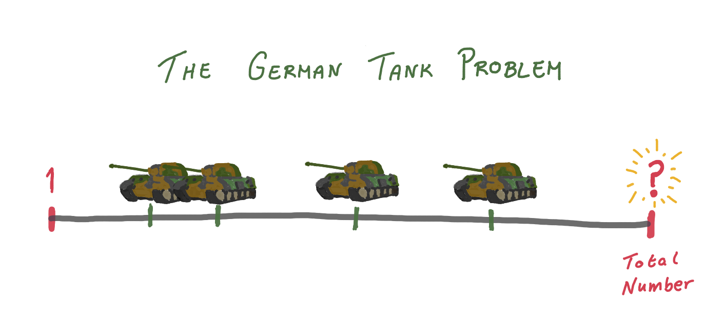
In the statistical theory of estimation, the German tank problem consists of estimating the maximum of a discrete uniform distribution from sampling without replacement. In simple terms, suppose there exists an unknown number of items which are sequentially numbered from 1 to N .
en.wikipedia.org/wiki/German_tank_…
What was the German tank problem in World War 2?
What was the German tank problem in World War 2?
[ [AdMiddle] Let’s take a trip back in time and look at what’s known as the “German tank problem” from World War II. At that time, for fairly obvious reasons, allied forces wanted to know how many tanks the German military was producing.
www.quickanddirtytips.com/education/math…
What is the formula for the German tank problem?
What is the formula for the German tank problem?
Introduction Mathematical Preliminaries GTP: Original GTP: New Regression References Appendix The German Tank Problem: Mathematical Formulation Original formulation: Tanks numbered from 1 to N, observe k, largest seen is m, estimate N with Nb=Nb(m,k).
web.williams.edu/Mathematics/sjmiller/publi…
Who is the author of the German tank problem?
Who is the author of the German tank problem?
The German Tank Problem: Math/Stats at War! Steven J. Miller: Carnegie Mellon and Williams College (sjm1@williams.edu, stevenm1@andrew.cmu.edu) http://www.williams.edu/Mathematics/sjmiller University of Connecticut Awards Dinner, April 26, 2019 1 Introduction Mathematical Preliminaries GTP: Original GTP: New Regression References Appendix
web.williams.edu/Mathematics/sjmiller/publi…
How many tanks did the Germans produce per month?
How many tanks did the Germans produce per month?
Pretty cool, right? And the statistical approach worked very well. Using traditional techniques (like spying and decoding encrypted messages), allied intelligence estimated that the Germans were producing about 1400 tanks per month.
www.quickanddirtytips.com/education/math…
https://en.m.wikipedia.org/wiki/German_tank_problem
Ориентировочное время чтения: 9 мин
In the statistical theory of estimation, the German tank problem consists of estimating the maximum of a discrete uniform distribution from sampling without replacement. In simple terms, suppose there exists an unknown number of items which are sequentially numbered from 1 to N. A random sample of these items is taken and their sequence numbers observed; the problem is to estimate N f…
In the statistical theory of estimation, the German tank problem consists of estimating the maximum of a discrete uniform distribution from sampling without replacement. In simple terms, suppose there exists an unknown number of items which are sequentially numbered from 1 to N. A random sample of these items is taken and their sequence numbers observed; the problem is to estimate N from these observed numbers.

The problem can be approached using either frequentist inference or Bayesian inference, leading to different results. Estimating the population maximum based on a single sample yields divergent results, whereas estimation based on multiple samples is a practical estimation question whose answer is simple (especially in the frequentist setting) but not obvious (especially in the Bayesian setting).

The problem is named after its historical application by Allied forces in World War II to the estimation of the monthly rate of German tank production from very limited data. This exploited the manufacturing practice of assigning and attaching ascending sequences of serial numbers to tank components (chassis, gearbox, engine, wheels), with some of the tanks eventually being captured in battle by Allied forces.
https://www.albert.io/blog/german-tank-problem-explained-ap-statistics-review
What Is The German Tank Problem?
The Problem with Samples and Estimators
How to Use The Minimum-Variance Unbiased Estimator
Wrapping Up The German Tank Question
The German Tank Problem is a famous statistical problem that helped the Allied Forces during World War II, and can help you with your AP® Statistics review. Statisticians use estimatorswhen dealing with samples from a larger population. Often, it can be useful to know the size of the total population wh…
Задача о немецких танках — задача статистической теории оценивания по определению величины …
Дискретное равномерное распределение
Текст из Википедии, лицензия CC-BY-SA
https://web.williams.edu/Mathematics/sjmiller/public_html/math/talks/GermanTankProblem...
The German Tank Problem: Mathematical Formulation Original formulation: Tanks numbered from 1 to N, observe k, largest seen is m, estimate N with Nb=Nb(m,k). New version: Tanks …
https://brilliant.org/problems/german-tank-problem
Перевести · German Tank Problem Probability Level 2 An airline has numbered their planes 1 , 2 , … , N , 1,2,\ldots,N, 1 , 2 , … , N , and you …
https://www.eadan.net/blog/german-tank-problem
Simulations
Our First Estimator
A Better Estimator
Where Do These Estimators Come from?
Probabilistic Programming
Let’s suppose there are 1,000 tanks in total, numbered sequentially from 1 to 1000, and we captured 15 of these tanks uniformly at random. Simulations are a nice way to build intu…
stat88.org/textbook/notebooks/Chapter_11/02_German_Tank_Problem_Revisited.html
Перевести · The German Tank Problem, Revisited Earlier in the course we examined the German tank problem in which statisticians helped the Allies estimate the number of tanks the Germans …
https://www.quickanddirtytips.com/.../math/how-statistics-solved-the-german-tank-problem
Перевести · 19.11.2010 · The German Tank Problem. [ [AdMiddle] Let’s take a trip back in time and look at what’s known as the “German tank problem” from World War II. At that time, for fairly obvious reasons, allied forces wanted to know how many tanks the German …
РекламаСтрептокарпусы польской и российской селекции. Доставка по России.
РекламаКрасивые букеты от 1 550 руб. Доставка 0 руб. по Москве. Работаем 24/7. Заказать! · Москва · пн-пт круглосуточно
Не удается получить доступ к вашему текущему расположению. Для получения лучших результатов предоставьте Bing доступ к данным о расположении или введите расположение.
Не удается получить доступ к расположению вашего устройства. Для получения лучших результатов введите расположение.

In the statistical theory of estimation, the German tank problem consists of estimating the maximum of a discrete uniform distribution from sampling without replacement. In simple terms, suppose there exists an unknown number of items which are sequentially numbered from 1 to N. A random sample of these items is taken and their sequence numbers observed; the problem is to estimate N from these observed numbers.
The problem can be approached using either frequentist inference or Bayesian inference, leading to different results. Estimating the population maximum based on a single sample yields divergent results, whereas estimation based on multiple samples is a practical estimation question whose answer is simple (especially in the frequentist setting) but not obvious (especially in the Bayesian setting).
The problem is named after its historical application by Allied forces in World War II to the estimation of the monthly rate of German tank production from very limited data. This exploited the manufacturing practice of assigning and attaching ascending sequences of serial numbers to tank components (chassis, gearbox, engine, wheels), with some of the tanks eventually being captured in battle by Allied forces.
The adversary is presumed to have manufactured a series of tanks marked with consecutive whole numbers, beginning with serial number 1. Additionally, regardless of a tank's date of manufacture, history of service, or the serial number it bears, the distribution over serial numbers becoming revealed to analysis is uniform, up to the point in time when the analysis is conducted.
Assuming tanks are assigned sequential serial numbers starting with 1, suppose that four tanks are captured and that they have the serial numbers: 19, 40, 42 and 60.
The frequentist approach predicts the total number of tanks produced will be:
The Bayesian approach predicts that the median number of tanks produced will be very similar to the frequentist prediction:
whereas the Bayesian mean predicts that the number of tanks produced would be:
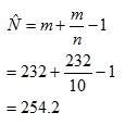
Let N equal the total number of tanks predicted to have been produced, m equal the highest serial number observed and k equal the number of tanks captured.
The frequentist prediction is calculated as:
The Bayesian median is calculated as:
The Bayesian mean is calculated as:
Both Bayesian computations are based on the following probability mass function:
This distribution has a positive skewness, related to the fact that there are at least 60 tanks. Because of this skewness, the mean may not be the most meaningful estimate. The median in this example is 74.5, in close agreement with the frequentist formula. Using Stirling's approximation, the Bayesian probability function may be approximated as
which results in the following approximation for the median:
Finally, the average estimate by Bayesians, and its deviation, are computed as:
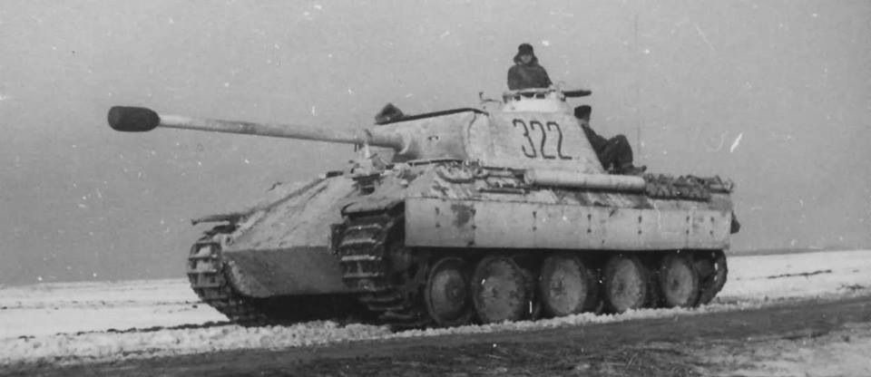
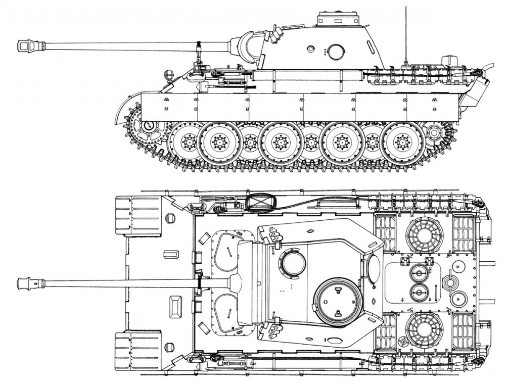
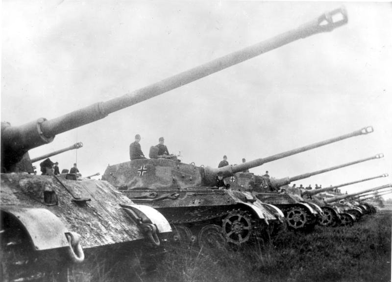
During the course of the Second World War, the Western Allies made sustained efforts to determine the extent of German production and approached this in two major ways: conventional intelligence gathering and statistical estimation. In many cases, statistical analysis substantially improved on conventional intelligence. In some cases, conventional intelligence was used in conjunction with statistical methods, as was the case in estimation of Panther tank production just prior to D-Day.
The allied command structure had thought the Panzer V (Panther) tanks seen in Italy, with their high velocity, long-barreled 75 mm/L70 guns, were unusual heavy tanks and would only be seen in northern France in small numbers, much the same way as the Tiger I was seen in Tunisia. The US Army was confident that the Sherman tank would continue to perform well, as it had versus the Panzer III and Panzer IV tanks in North Africa and Sicily.[a] Shortly before D-Day, rumors indicated that large numbers of Panzer V tanks were being used.
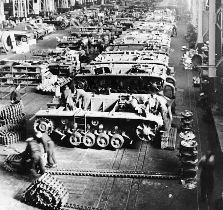
To determine whether this was true, the Allies attempted to estimate the number of tanks being produced. To do this, they used the serial numbers on captured or destroyed tanks. The principal numbers used were gearbox numbers, as these fell in two unbroken sequences. Chassis and engine numbers were also used, though their use was more complicated. Various other components were used to cross-check the analysis. Similar analyses were done on wheels, which were observed to be sequentially numbered (i.e., 1, 2, 3, ..., N).[2][page needed][b][3][4]
The analysis of tank wheels yielded an estimate for the number of wheel molds that were in use. A discussion with British road wheel makers then estimated the number of wheels that could be produced from this many molds, which yielded the number of tanks that were being produced each month. Analysis of wheels from two tanks (32 road wheels each, 64 road wheels total) yielded an estimate of 270 tanks produced in February 1944, substantially more than had previously been suspected.[5]
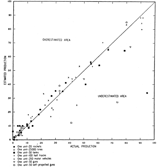
German records after the war showed production for the month of February 1944 was 276.[6][c] The statistical approach proved to be far more accurate than conventional intelligence methods, and the phrase "German tank problem" became accepted as a descriptor for this type of statistical analysis.
Estimating production was not the only use of this serial-number analysis. It was also used to understand German production more generally, including number of factories, relative importance of factories, length of supply chain (based on lag between production and use), changes in production, and use of resources such as rubber.
According to conventional Allied intelligence estimates, the Germans were producing around 1,400 tanks a month between June 1940 and September 1942. Applying the formula below to the serial numbers of captured tanks, the number was calculated to be 246 a month. After the war, captured German production figures from the ministry of Albert Speer showed the actual number to be 245.[3]
Estimates for some specific months are given as:[7]
Similar serial-number analysis was used for other military equipment during World War II, most successfully for the V-2 rocket.[8]
Factory markings on Soviet military equipment were analyzed during the Korean War, and by German intelligence during World War II.[9]
In the 1980s, some Americans were given access to the production line of Israel's Merkava tanks. The production numbers were classified, but the tanks had serial numbers, allowing estimation of production.[10]
The formula has been used in non-military contexts, for example to estimate the number of Commodore 64 computers built, where the result (12.5 million) matches the low-end estimates.[11]
To confound serial-number analysis, serial numbers can be excluded, or usable auxiliary information reduced. Alternatively, serial numbers that resist cryptanalysis can be used, most effectively by randomly choosing numbers without replacement from a list that is much larger than the number of objects produced, or by producing random numbers and checking them against the list of already assigned numbers; collisions are likely to occur unless the number of digits possible is more than twice the number of digits in the number of objects produced (where the serial number can be in any base); see birthday problem.[d] For this, a cryptographically secure pseudorandom number generator may be used. All these methods require a lookup table (or breaking the cypher) to back out from serial number to production order, which complicates use of serial numbers: a range of serial numbers cannot be recalled, for instance, but each must be looked up individually, or a list generated.
Alternatively, sequential serial numbers can be encrypted with a simple substitution cipher, which allows easy decoding, but is also easily broken by frequency analysis: even if starting from an arbitrary point, the plaintext has a pattern (namely, numbers are in sequence). One example is given in Ken Follett's novel Code to Zero, where the encryption of the Jupiter-C rocket serial numbers is given by:
The code word here is Huntsville (with repeated letters omitted) to get a 10-letter key.[12] The rocket number 13 was therefore "HN", and the rocket number 24 was "UT".
Strong encryption of serial numbers without expanding them can be achieved with format-preserving encryption. Instead of storing a truly random permutation on the set of all possible serial numbers in a large table, such algorithms will derive a pseudo-random permutation from a secret key. Security can then be defined as the pseudo-random permutation being indistinguishable from a truly random permutation to an attacker who doesn't know the key.
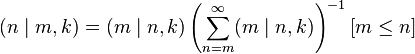
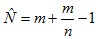
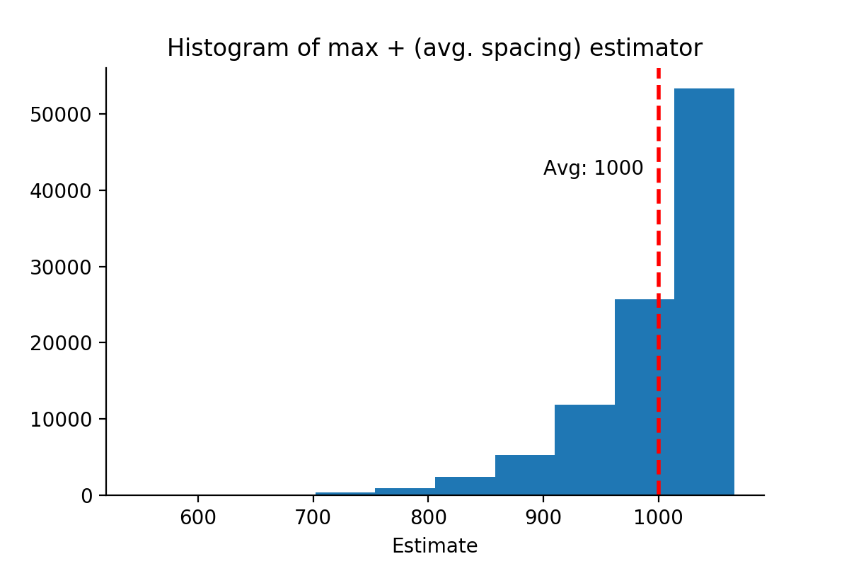
For point estimation (estimating a single value for the total, ), the minimum-variance unbiased estimator (MVUE, or UMVU estimator) is given by:[e]
where m is the largest serial number observed (sample maximum) and k is the number of tanks observed (sample size).[10][13] Note that once a serial number has been observed, it is no longer in the pool and will not be observed again.
so the standard deviation is approximately N/k, the expected size of the gap between sorted observations in the sample.
The formula may be understood intuitively as the sample maximum plus the average gap between observations in the sample, the sample maximum being chosen as the initial estimator, due to being the maximum likelihood estimator,[f] with the gap being added to compensate for the negative bias of the sample maximum as an estimator for the population maximum,[g] and written as
This can be visualized by imagining that the observations in the sample are evenly spaced throughout the range, with additional observations just outside the range at 0 and N + 1. If starting with an initial gap between 0 and the lowest observation in the sample (the sample minimum), the average gap between consecutive observations in the sample is ; the being because the observations themselves are not counted in computing the gap between observations.[h]. A derivation of the expected value and the variance of the sample maximum are shown in the page of the discrete uniform distribution.
This philosophy is formalized and generalized in the method of maximum spacing estimation; a similar heuristic is used for plotting position in a Q–Q plot, plotting sample points at k / (n + 1), which is evenly on the uniform distribution, with a gap at the end.
Instead of, or in addition to, point estimation, interval estimation can be carried out, such as confidence intervals. These are easily computed, based on the observation that the probability that k observations in the sample will fall in an interval covering p of the range (0 ≤ p ≤ 1) is pk (assuming in this section that draws are with replacement, to simplify computations; if draws are without replacement, this overstates the likelihood, and intervals will be overly conservative).
Thus the sampling distribution of the quantile of the sample maximum is the graph x1/k from 0 to 1: the p-th to q-th quantile of the sample maximum m are the interval [p1/kN, q1/kN]. Inverting this yields the corresponding confidence interval for the population maximum of [m/q1/k, m/p1/k].
For example, taking the symmetric 95% interval p = 2.5% and q = 97.5% for k = 5 yields 0.0251/5 ≈ 0.48, 0.9751/5 ≈ 0.995, so the confidence interval is approximately [1.005m, 2.08m]. The lower bound is very close to m, thus more informative is the asymmetric confidence interval from p = 5% to 100%; for k = 5 this yields 0.051/5 ≈ 0.55 and the interval [m, 1.82m].
More generally, the (downward biased) 95% confidence interval is [m, m/0.051/k] = [m, m·201/k]. For a range of k values, with the UMVU point estimator (plus 1 for legibility) for reference, this yields:
Note that m/k cannot be used naively (or rather (m + m/k − 1)/k) as an estimate of the standard error SE, as the standard error of an estimator is based on the population maximum (a parameter), and using an estimate to estimate the error in that very estimate is circular reasoning.
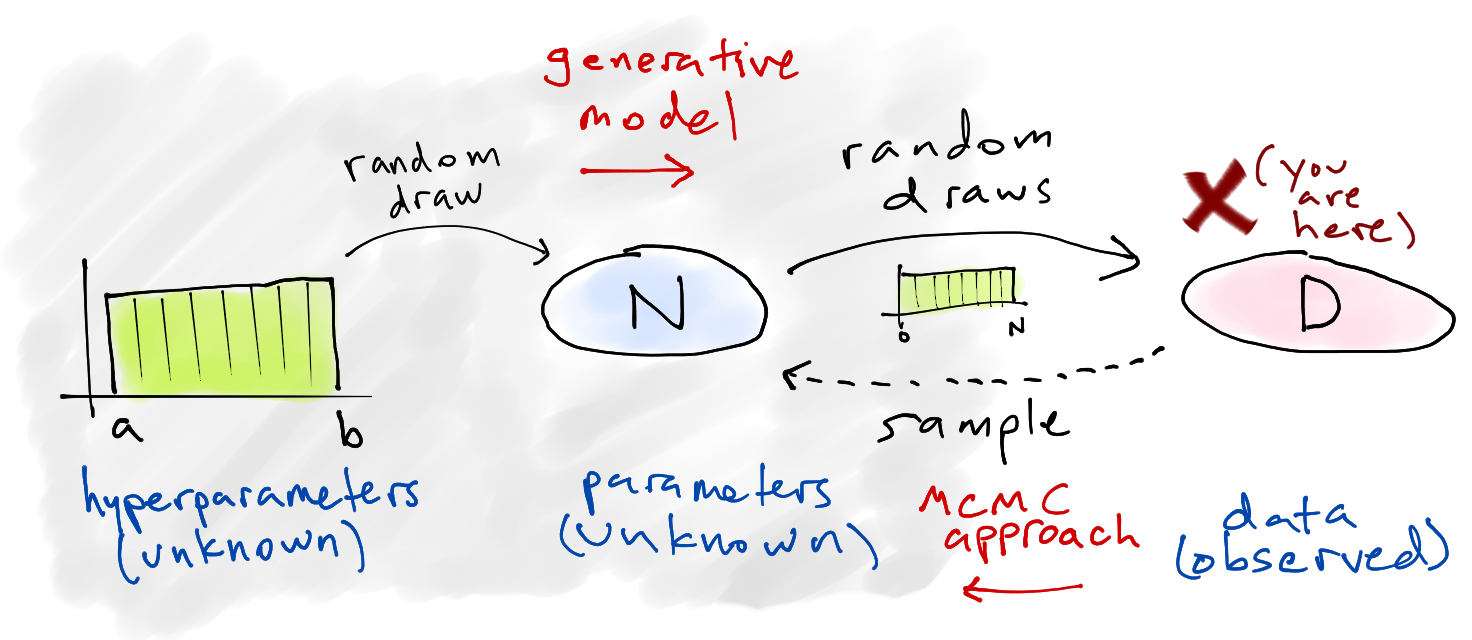
The Bayesian approach to the German tank problem is to consider the credibility that the number of enemy tanks is equal to the number , when the number of observed tanks, is equal to the number , and the maximum observed serial number is equal to the number . The answer to this problem depends on the choice of prior for .
Pussy Teen Nature No Nude
Shemale Teen Hard
Girls Stripping All The Way Naked
California Girl Bikini Contest
Big Ass Teens Interracial
German tank problem - Wikipedia
The German Tank Problem Explained: AP® Statistics Review
The German Tank Problem: Math/Stats at War!
German Tank Problem - Brilliant
The German Tank Problem - eadan.net
The German Tank Problem, Revisited - Stat 88
How Statistics Solved the German Tank Problem
German Tank Problem